![]()
Frontline Learning Research Vol.11 No. 2 (2023) 1 - 30
ISSN 2295-3159
1Utrecht University, The Netherlands
2University of Applied Science Utrecht, the Netherlands
3Middlebury College, Middlebury, VT, USA
*These authors share first authorship
Article received 25 July 2022/ revised 22 June 2023/ accepted 27 June 2023/ available online 5 September 2023
Many students persistently misinterpret histograms. Literature suggests that having students solve dotplot items may prepare for interpreting histograms, as interpreting dotplots can help students realize that the statistical variable is presented on the horizontal axis. In this study, we explore a special case of this suggestion, namely, how students’ histogram interpretations alter during an assessment. The research question is: In what way do secondary school students’ histogram interpretations change after solving dotplot items? Two histogram items were solved before solving dotplot items and two after. Students were asked to estimate or compare arithmetic means. Students’ gaze data, answers, and cued retrospective verbal reports were collected. We used students’ gaze data on four histogram items as inputs for a machine learning algorithm (MLA; random forest). Results show that the MLA can quite accurately classify whether students’ gaze data belonged to an item solved before or after the dotplot items. Moreover, the direction (e.g., almost vertical) and length of students’ saccades were different on the before and after items. These changes can indicate a change in strategies. A plausible explanation is that solving dotplot items creates readiness for learning and that reflecting on the solution strategy during recall then brings new insights. This study has implications for assessments and homework. Novel in the study is its use of spatial gaze data and its use of an MLA for finding differences in gazes that are relevant for changes in students’ task-specific strategies.
Keywords: Statistics Education; Histogram and Dotplot; Eye-Tracking; Random Forest; Practice Effect
Statistical literacy includes “people’s ability to interpret and critically evaluate statistical information, data-related arguments […], which they may encounter in diverse contexts, and when relevant” (Gal, 2002, p. 4; emphasis in original). As data consumers, citizens should be able to correctly interpret various graphical displays. This is particularly important in this era of vague and fake news “that place interpretive and evaluative demands on a reader or viewer” (Gal & Geiger, 2022, p. 2). In this study, we specifically focus on the graphical representation of histograms.
Histograms can reveal particular aspects of the distribution of the data often hidden in other graphs (e.g., Pastore et al., 2017). Furthermore, as histograms are ubiquitous in research and education, they need to be learned (cf. Garfield & Ben-Zvi, 2008). For example, searching for ‘histogram’ in Google Scholar resulted in more than 3.2 million hits (June 13, 2023). Therefore, the guidelines for assessment and instruction in statistics education II (GAISE II) for all Grades up to Grade 12 contain several examples of histograms and dotplots (for levels A, B, and C), with levels B and C roughly corresponding to middle and high school (Bargagliotti et al., 2020). Moreover, some alternatives for histograms, such as boxplots, are even more complex (e.g., Bakker et al., 2004).
However, many people persistently misinterpret histograms (e.g., Cooper, 2018; Kaplan, 2014). For example, Bakker (2004a) found that secondary school students (Grades 7–8) considered the individual heights of bars in a histogram to be the heights of individual people, rather than aggregations of data. Students’ conceptual difficulties with histograms are well documented (e.g., Boels, Bakker, Van Dooren & Drijvers, 2019), but it is unclear how to support students in learning to interpret histograms.
Figure 1. Example of dotplot Item17 that required students to compare two datasets regarding their mean.
Several studies suggest that having students solve dotplot items can scaffold this learning (e.g., delMas & Liu, 2005; Garfield & Ben-Zvi, 2008; Makar & Confrey, 2004). In most of these studies, students’ answers and verbal reports were the main sources of information. Dotplots have the advantage that they show all individual data points as well as their distribution (Figures 1, 2). In addition, the absence of a vertical scale in dotplots can turn students’ attention toward the horizontal scale, which is where the variable is presented in both graphs. However, little is known about whether solving dotplot items allows students to become aware of aspects of graph representation and statistical variables that are useful for interpreting histograms. The aim of this study is, therefore, to explore how solving dotplot items influences secondary school students’ thinking on a detailed level when they interpret histograms. Our overall research question is: In what way do secondary school students’ histogram interpretations change after solving dotplot items? In the Theoretical Background section, we will specify this overall question with three sub-questions.
As we elaborate further in the Theoretical Background section, gaze data can reveal students’ strategies in real-time, and in more detail, compared to concurrent thinking aloud (verbal reports) and without the risk of influencing the thinking process (Van Gog et al., 2005; Van Gog & Jarodzka, 2013). We use students’ gaze data when solving four items with histograms before and after solving similar items with dotplots, as well as their answers on these items. The four histogram items were taken from a larger sequence with 25 digital items in total. Furthermore, we examined transcripts from stimulated recall (Lyle, 2003) verbal reports about students’ strategies (for more details see section 3.3.2). In the next section, we elaborate on difficulties with histograms and dotplots and discuss how gaze data can be used.
Figure 2. Example of a dotplot (left) and a histogram (right) depicting the same distribution.
Note. The dotplot was part of Item16. The histogram was part of Item05, not further discussed here (for more details, see Boels, Bakker, et al., 2022).
In this section, we review statistics education literature on the problem (many students persistently misinterpret histograms), a gap in this literature (the variation in results on students’ interpretations of dotplots), and graphs that are suggested for supporting students in learning to interpret histograms.
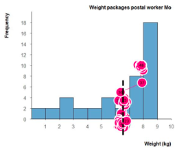
Figure 3. An example of a histogram.
Note. The measured variable (weight) is along the horizontal axis. The weights of 67 packages (sum of frequencies) are depicted in this histogram. The arithmetic mean weight is 3.3 kg.
2.1.1 Histograms are Persistently Misinterpreted
Many people persistently misinterpret histograms (e.g., Cohen, 1996; Setiawan & Sukoco, 2021). Researchers and teachers think that there is no difference between bar graphs and histograms (e.g., Clayden & Croft, 1990; Tiefenbruck, 2007). Dabos (2014) found that some college teachers did not see when students incorrectly counted the number of bars in a histogram to get the total frequency instead of adding the bars’ heights. First-year university students in educational sciences had difficulties finding or interpreting the mean, median, variation, and skewness in histograms (Lem et al., 2013). College students interpreted the horizontal salary scale in a histogram as a timescale (Meletiou, 2000). Middle school students used unequal intervals in a histogram with frequency on the vertical axis—instead of density—hence, not correcting the frequencies for unequal bin widths (McGatha et al., 2002). Other middle school students thought that bars in histograms are connected for easier comparison (e.g., Capraro et al., 2005). Students in Grades 6–12 answered histogram items 17% to 53% correctly on average (Whitaker & Jacobbe, 2017). Many students mistakenly took bars’ heights as the measured value. Such students possibly think that only nine packages are depicted in the histogram in Figure 3 (the number of bars) instead of 67 (the actual number).
2.1.2 Dotplots are not always Correctly Interpreted
Generally, dotplots are interpreted better than histograms (e.g., delMas et al., 2005), although stacked dotplots (in the early days also called line plots; e.g., Tiefenbruck, 2007) might still confuse students (e.g., Lyford, 2017). Lem et al. (2013) found that university students understood dotplots slightly better than histograms (on average, 55% correct responses for dotplots versus 51% for histograms). However, in that study, two dotplot items scored worse. University students taking introductory statistics explored variability and standard deviation through a kind of stacked dotplots (delMas & Liu, 2005). Most of these students did not fully understand how standard deviation was related to the distribution of data in a histogram.
Figure 4. Example of a double dotplot.
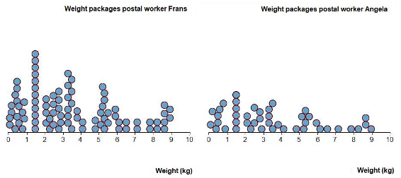
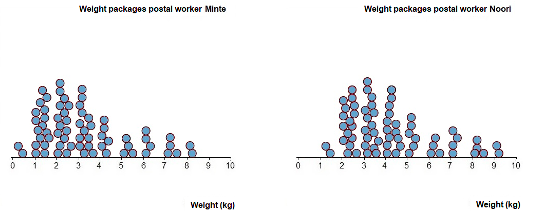
Note. This was Item14 in the original sequence of 25 digital items. The question was: ‘Which postal worker delivers the heaviest packages on average?’ with three answer options: (a) Frans delivers the heaviest packages on average, (b) Angela delivers the heaviest packages on average, and (c) The mean weight for both is approximately the same. The correct answer here is (c).
A local instruction theory in statistics education suggests that dotplots are suitable for supporting students’ learning of distribution and variability in data represented in histograms (e.g., Bakker & Gravemeijer, 2004; Garfield, 2002). Garfield & Ben-Zvi (2008) stated: “studies [that] suggest a sequence of activities that leads students from […] dotplots […] to histograms” can support students in “developing the concept of distribution as an entity” (p. 175). An advantage of dotplots over histograms is that dotplots show the distribution of data in a disaggregated form. In addition, dotplots can draw students’ attention to the variable being depicted along the horizontal axis—similar to histograms—, as dotplots have only this axis. A possible disadvantage of dotplots for teaching students to interpret histograms (aggregated data) is that dotplots might invite them to see the data as individual cases (Konold et al., 2015) instead of looking at aggregated measures (including arithmetic mean).
One explanation for dotplots sometimes being misinterpreted is that students do not understand where the measured values are depicted in stacked dotplots due to the countable height of the stack. Hence, students confuse frequency—the height of the bar or stack—with the measured value (e.g., Cooper & Shore, 2008; Cooper 2018, Kaplan et al., 2014), similar to histograms. For stacked dotplots, a vertical axis is possible but not necessary, which might induce this same height misinterpretation (e.g., Lyford, 2017). Some of the previously described persistent misinterpretations with histograms are related to the data in a histogram; more specifically:
In non-stacked dotplots, no variable is represented in the vertical direction (see Figures 1, 2, and 4). Therefore, non-stacked dotplots have the potential to raise students’ awareness of the variable (here: weight) being depicted along the horizontal axis in dotplots and histograms. Nevertheless, abstract dotplots without context or numbers along the horizontal axis can lead to misinterpretations of variability (Kaplan et al., 2014). The same may hold for axis titles that are missing (such as in Lem et al., 2013). Thus, we use context, an axis title, and numbers in our dotplots. We conjecture that these non-stacked (‘messy’) dotplots support students’ histogram interpretations. Therefore, as stated in the introduction, our overall research question is: In what way do secondary school students’ histogram interpretations change after solving dotplot items?
In this section, we review what is already known from gaze data in education and what measures are most suitable for our aim. In addition, we elaborate on how gaze data can be connected to students’ strategies. We end each section with a sub-question.
2.2.1 Use of Spatial Gaze Measures to Reveal Students’ Strategies for Interpreting Histograms
The use of gaze data for studying learning is not new (e.g., Strohmaier et al., 2020). For example, Garcia Moreno-Esteva et al. (2018) and Khalil (2005) studied students’ visual cognitive behaviors on statistical graphs. A main advantage of eye-tracking “is that it can provide detailed information about the time-course of processing” (Kaakinen, 2021, p. 170). Most studies neglect this level of detail by using gaze data measures that are temporal (e.g., total fixation duration, reaction times), count (fixation count, number of saccades between relevant or irrelevant parts of the stimuli), or both (e.g., Kaakinen, 2021; Lai et al., 2013). Traditional time measures, for example, can hide visual scanning patterns (Goldberg & Helfman, 2010). A similar argumentation can be made for count measures such as the percent of fixations on specific parts of the screen (Godau et al., 2014).
Spatial measures, such as a sequence of Areas of Interest (AOIs, e.g., Garcia Moreno-Esteva et al., 2018, 2020) can disclose the kind of detailed information Kaakinen (2021) refers to. Spatial measures, such as scanpaths, seem better suited for providing detailed information about students’ thinking (Hyönä, 2010). Dewhurst et al. (2018) were one of the first who studied (simplified) scanpaths using vectors in (scene) viewing tasks. Their vectors include the direction and magnitude of saccades.
In a previous study, we qualitatively analyzed students’ scanpath patterns (sequence of fixations and saccades) when students estimated the mean from histograms (Boels, Bakker & Drijvers, 2019). After qualitatively coding 300 videos with students’ gazes and verbal reports of 25 students in that study, we found that the perceptual form of students’ scanpath patterns within one AOI—the graph area—was most relevant for students’ task-specific strategies on these items, see Figure 5. This perceptual form can be captured by the direction (angle) and magnitude (length) of students’ saccades.
In that study, we found several scanpath patterns that were indicative of students’ task-specific strategies. All patterns were found on the graph area only. In one pattern, the perceptual form of that pattern was identified as vertical if successive saccades on the graph area were vertical and roughly aligned with each other (Figure 5). This vertical scanpath pattern indicates that this student (correctly) tried to find the balancing point of the graph as an estimation of the mean. Another scanpath pattern was a horizontal gaze pattern indicating that this student (incorrectly) tried to make all bars equally high which resulted in the mean of the frequencies instead of the mean weight. In total, five different scanpath patterns were found for students estimating and comparing means of histograms, each related to a specific strategy (Boels, Bakker, et al., 2022). Other AOIs did not emerge as relevant to these students’ task-specific strategies.
Figure 5. Example of a vertical scanpath on Item 20.
Note. Circles indicate fixations (positions on the screen where students look longer), and thin lines between the circles indicate saccades (fast transitions between two fixations). A vertical line segment—indicating a scanpath—is superimposed for the reader’s convenience. A scanpath is a sequence of fixations and saccades. “A fixation is a period of time during which a specific part of [the computer screen] is looked at and thereby projected to a relatively constant location on the retina. This is operationalized as a relatively still gaze position in the eye-tracker signal implemented using the [Tobii] algorithm.” (Hessels et al., 2018, p. 22). (The figure has been translated into English.)
As the overall research question for this study indicates, we want to explore in what way secondary school students learn from dotplot items. Given that the scanpath patterns on the graph area indicate students’ strategies, we examine differences in these patterns on histogram items before and after students solved items with dotplots. We only address the main differences, those being differences relevant to students’ task-specific strategies. The first sub-question for the present study is, therefore:
1) What are the main differences in students’ gaze patterns on histogram items before and after solving dotplot items?
2.2.2 Connecting Gaze Data to Students’ Strategies
Although scanpaths can reveal students’ strategies on a detailed level, there is no simple relation between eye movements and strategies (e.g., Orquin & Holmqvist, 2017; Russo, 2010) as not every eye movement is part of a task-specific strategy (e.g., Schindler & Lilienthal, 2019). Therefore, it is often needed to also ask at least some students what approach they took to solve the items.
Instead of concurrent think-aloud protocols, recalls (retrospective reports) are preferred for complex items (e.g., Van Gog et al., 2005) as concurrent thinking aloud may influence both eye movements and students’ thinking (Van Gog & Jarodzka, 2013). The disadvantage of such retrospective think-aloud reports, however, is that students may have forgotten their strategy after completing all items. This risk can be reduced by having students look back at their eye movements (e.g., Guan et al., 2006; Kragten et al., 2015; Van Gog et al., 2005). Therefore, in the stimulated recall (cued retrospective reports), we individually cued each student with their own gazes. How we did that, is explained in the data collection section. The second sub-question for the present study is:
2) What indications can be found in students’ verbalizations during stimulated recall that changes in their approaches to histograms occurred?
Students learning from a sequence of tasks is known as the practice, test-retest, or retesting effect in assessment theories (e.g., Heilbronner et al., 2010; Scharfen et al., 2018). The practice effect refers to improved performance (often scores or answers) due to repeated assessment with the same or similar, equally difficult items. The time interval between two assessments can be very short—5 or 10 minutes—to find such an effect (e.g., Catron, 1978; Falleti et al., 2006). The practice effect was found for several general cognitive function assessments for items that required memorization (e.g., of numbers), change detection (e.g., of changed colors between two items), and matching (e.g., what parts of items are alike). In addition, familiarity with test requirements can cause differences between the test and retest results (e.g., Falleti et al., 2006) and reduce anxiety (e.g., Catron, 1978). Furthermore, regression to the mean can cause extreme results—high and low performance scores—to come closer to the mean, resulting in both under- and overestimation of improvement (e.g., Temkin et al., 1999). For achievement or knowledge tests, such as formative assessments in secondary education, the practice effect is also associated with actual or true learning as opposed to most cognitive tests, for example, IQ tests, for which learning is unlikely to occur (e.g., Lievens et al., 2007; Scharfen et al., 2018). Lumsden suggested that the practice effect can also be found within a sequence of items (1976). In addition, gaze data have been used to examine the practice effect (e.g., Guerra-Carrillo & Bunge, 2018; Płomecka et al., 2020). Although this is not the focus of our study, to the best of our knowledge, our study is the first that looks at a within-a-sequence-of-items practice effect.
Most research investigating the practice effect uses scores on standardized tests (e.g., in this meta-analysis: Hinton-Bayre, 2010). However, standardized tests often lack instructional relevance (e.g., Hohn, 1992). Practitioners, such as mathematics teachers, are more interested in knowing whether students learn from a low-stake sequence of items. Moreover, teachers are interested in students’ strategies, hence “gaining qualitative insight into student understanding” (Bennett, 2011, p. 6). In this study, we, therefore, examine students’ changes in strategies during solving items as an indication of potential learning. To exclude several other possible influencing factors—such as peers’ or teachers’ interventions—we use items from one sequence of items with statistical graphs.
For some items, students verbally reported their answer (estimation of the arithmetic mean), while for other items, they chose one of three answer options (comparing means, Figure 4). If a change in students’ strategies occurred toward a correct instead of an incorrect strategy, we would also expect a difference in students’ answers, including answer correctness. Therefore, the third sub-question for this research is:
What are the differences in students’ answers on histogram items before and after solving dotplot items?
For very small data sets or very short sequences of tasks, the first sub-research question could theoretically be answered through the careful, manual study of gaze data. Our study, however, seeks to use machine learning to both augment the effectiveness of identifying differences in students’ gaze patterns between items and to identify these differences at a scale that would be impractical to do by hand. To build an analytical model of the gazes, a non-ML approach could be used. The ones we tried (e.g., logistic regression) performed relatively poorly (see also Lyford & Boels, 2022). Instead, we use supervised learning, a subset of MLAs that use training data and pattern recognition to predict a well-defined output (Friedman et al., 2001). In particular, the present study uses the random forests algorithm (Breiman, 2001), which will allow us to effectively and efficiently identify systemic differences in gazes between our two hundred student-item pairings. These random forests can not only be efficiently trained and used to identify patterns in students’ gaze data, but they are also likely to identify systematic differences in gaze data that are unnoticeable upon manual inspection (James et al., 2013). In addition, through assessing the importance of specific variables (Figure 15), random forests allow for some interpretability so that researchers can better understand what some of the differences in gazes might be (e.g., proportionally more vertical instead of more horizontal gazes could indicate a change from an incorrect to a correct strategy), and postulate about possible mechanisms.
Details on participants, the eye-tracking method, and two items (Item02 and Item11) were reported previously in a qualitative study (Boels, Bakker, et al., 2022). Two items were used previously in a machine learning analysis (Item02 and Item20; Boels, Garcia Moreno-Esteva, et al., accepted) but with a different aim, namely, to examine how a machine learning algorithm (MLA) could identify students that used a correct or incorrect strategy—for solving the item—purely based on their gaze data on the graph area of this item. For the reader’s convenience, we here summarize all information relevant to the present study.
Participants were 50 Grades 10–12 pre-university track students from a Dutch public secondary school [15–19 years old; mean = 16.31 years]; 23 males, 27 females (more details in Table 1). In the Netherlands, secondary school students are in a pre-vocational, pre-college, or pre-university track. Generally speaking, the pre-university track implies mostly high-performing students. All participants had statistics in their mathematics curriculum. Each student individually solved the items in a separate room in their school. Participation was voluntary; permission from the Utrecht University ethical committee was obtained, and informed consent was signed. Participants received a small gift for their participation.
Table 1
Grade level and age of participants. One participant did not provide details on grade, and another one did not provide age (see also Boels, Bakker, et al., 2022)
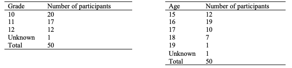
Note. Due to legislation, data on ethnicity cannot be collected. In the Netherlands, there is hardly any difference between public and private schools, nor between city, suburban, and rural schools. Private schools are rare.
3.2.1 Estimating and Comparing Arithmetic Means Reveals Students’ Knowledge
To reveal strengths and flaws in students’ knowledge about data in graphs such as histograms, Gal (1995) advises asking students to compute or estimate means from data in graphs. We, therefore, designed histogram and dotplot items that required students to estimate the arithmetic mean. This mean can be estimated from a histogram and dotplot by finding the equilibrium or balancing point from the graph (e.g., Mokros & Russell, 1995; O’Dell, 2012; see also Figure 5). In statistics, the mean is often used for comparing the data for two groups (e.g., Gal, 1995; Konold & Pollatsek, 2002). We, therefore, added items for which a comparison of means was needed (see Figure 4 for an example of a dotplot item that was used between the before and after histogram items).
3.2.2 Four Histogram Items—Dotplots Items in between
In the present study, we analyze students’ gaze data on four items from a sequence of items on a computer screen with several statistical graphs (Dataset1). We chose two item pairs from this sequence that are suitable for analysis with a machine learning algorithm, as these items are very similar, see Figure 6 (Dataset1, 5). Two items were given before a sequence of six dotplot items, and the other two afterward. Note that the after items are mirrored versions of the before items. The first pair of items we examine—before Item02 and after Item20—require students to estimate the mean of the data in one histogram. We will henceforth refer to these as ‘single-histogram’ items. The question for both items was: What is, approximately, the mean weight of the packages that [Anton/Mo] delivers? The second pair of items—before Item11 and after Item21—require students to compare the mean of the data in two histograms. We will henceforth refer to these as ‘double-histogram’ items. The question for both items was: Which postal worker delivers the heaviest packages on average? For each item, three answer options were given: (a) [Ellen/Elizabeth] delivers the heaviest packages on average, (b) [Titia/Monsif] delivers the heaviest packages on average, and (c) The mean weights for both are approximately the same. The correct answer for both items is (c).
Figure 6. Graphs of single-histogram items (left) and double-histogram items (middle and right) in the before (top row) and after (bottom row) versions.
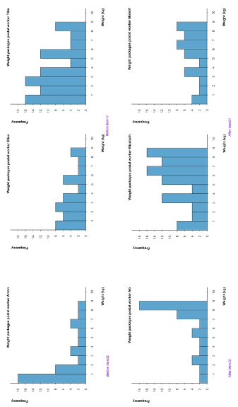
Note. Translated into English and numbering added. The numbering of the items (e.g., Item11) refers to the numbering in the original sequence of 25 digital items (Dataset1, Boels, Bakker, et al., 2022). Each after item (bottom row) is a mirrored version of the before item (top row).
Six of the items between the items before and after were non-stacked dotplots that were specifically designed to scaffold students (Items13–18 from the original data collection, e.g., Figures 1, 2, and 4, Dataset1, 5). As described in the Theoretical Background section, we used dotplots to draw students’ attention to specific features of the histograms that are important but might have been misunderstood.
Data from a previous qualitative study is re-used for this study (Boels, Bakker, et al., 2022). Data collection included students’ answers on each item, x- and y-coordinates of gaze data on the items through an eye tracker, and stimulated recall verbal reports. The collection of the gaze data and stimulated recall are briefly described in the following section. For more details, interested readers are referred to the original study.
3.3.1 Data Collection with an Eye Tracker
A Tobii XII-60 (sampling rate: 60 Hz) was placed on an HP-ProBook-6360b laptop between the 13-inch screen (refresh rate 59 Hz) and the keyboard, see Figure 7. Participants used a chin rest. Gaze data were recorded and processed with Tobii Studio software version 3.4.5 (Tobii, n.d.). Tobii software’s calibration procedure consisted of a 9-point calibration. As this software has no built-in validation procedure, we included a validation screen in the set-up at the beginning, after each item, and at the end (more details in Dataset1). We collected the raw data of the eye movements on each item (e.g., x- and y-coordinates of the eyes on the screen for each time stamp as well as to which AOI these coordinates belong, see Dataset1, 5, and Figure 8) through the Tobii software. We also collected students’ answers (verbal answers for single graph items, clicked multiple-choice option for double graph items).
Figure 7. Set-up of the experiment.
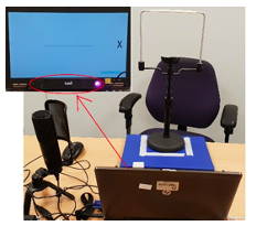
Note. For each participant, a chin rest was used. The eye tracker was placed on the laptop (see the red oval below the screen, copied into the figure for the convenience of the reader).
Figure 8. AOIs of before Item11 (left) and Item02 (right).
Note. Left: the graph area consists of the yellow and green areas named It11b_graph_L_Ellen and It11b_graph_r_Titia. Right: the graph area is the light blue area named It2_graph.
No students were excluded from the data set, as the data loss per trial (averaged over all 50 participants) and the data loss per participant (averaged over all 25 items from the original Dataset1) were below the exclusion point (34% or more). The mean accuracy is 56.6 pixels (1.16°) with the highest accuracy on the most relevant part for our study: the graph area (middle of the screen; 13.4 pixels or 0.27°). The average precision (0.58°) is considered good. More details on accuracy, precision, and the eye tracker can be found in Dataset3 and Boels, Bakker, et al. (2022) in line with advice from Holmqvist et al. (2022). The design of the complete sequence of items (25 items in total), including files used in the Tobii Studio software, AOI sizes, and output, are available from a data repository (Dataset1).
3.3.2 Data Collection through Stimulated Recall Verbal Reports
Stimulated recall (Lyle, 2003) is also known as “cued retrospective reporting” (Van Gog et al., 2005, p. 273). It is called retrospective “own-perspective video think-aloud with eye-tracking” (McIntyre, 2022, p.4) when used with a head-mounted eye tracker. The first part of the verbal reports consisted of cued retrospective think-aloud. This means that students watched videos of their own gazes laid over the items, while they explained their thinking when they solved the items. The stimulated recall took place after the students had solved all items of the sequence of 25 items (Dataset 1). During the second part of the verbal reports, clarifying questions were asked such as why they stated that their previously given answer was incorrect. In this second part, participants were also confronted with inconsistencies in their reports, such as differences between the answer given during recall and the answer during item solving. Time constraints influenced how many items could be questioned when students reported verbally. During this stimulated recall, we illuminated the location where students looked—through a kind of spotlight—and made the rest of the graph darker (see also Boels, Bakker, et al., 2022). We preferred this method over having students look back at their fixations (e.g., red dots) for two reasons. First, it prevents students from making different eye movements when looking back—and describing the corresponding strategy—instead of the strategy they initially used. Second, this makes visible the exact information that the learner has looked at, instead of the information being covered by, for example, a red dot (the fixation; e.g., Jarodzka et al., 2013).
We used different methods for analyzing our data. For the first sub-question about differences in gaze data, we analyzed our data through a machine learning algorithm (MLA). For the second sub-question about changes in students’ strategies, we coded transcripts of verbal reports (for the codebooks see, Boels, Bakker, et al., 2022). For the third sub-question about students’ answers, we explored changes in answers and answer correctness. In the remainder of this section, we elaborate on the analysis with a machine learning algorithm.
Studies usually only report on successful approaches. As a result, other researchers keep reinventing the wheel. For the first sub-question, we, therefore, decided to report both the MLA approaches we tried: our failed attempt to use time metrics as inputs for the MLA and a successful approach with spatial metrics. Before applying a machine learning algorithm, we first wanted to get a better understanding of the underlying data. Therefore, first, we plotted a graph using the time metric total fixation time per AOI (also known as total dwell time or total fixation duration). Next, we used this same time metric as input for training our MLA. This approach failed to produce an accurate MLA. Moreover, although this time metric is commonly used, recent literature strongly advises against using total dwell time (Orquin & Holmqvist, 2017). Second, we examined saccade directions and magnitudes (spatial metrics). Finally, using these spatial metrics as inputs for our MLA was successful, which is in line with the results of previous studies (Boels, Bakker, et al., 2022; Boels, Garcia Moreno-Esteva, et al., accepted). In the next section, we first describe how the MLA we used (random forest) works for those not familiar with MLAs and wanting to roughly understand these. Next, we describe how we applied the MLA in a failing approach using total dwell time (3.4.2), and in a successful approach using saccade direction and magnitude (3.4.3).
3.4.1 Gaze-Data Analysis through a Machine Learning Algorithm (Random Forest)
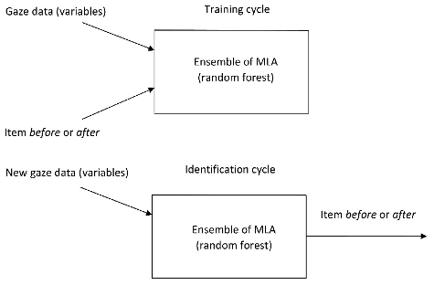
A machine learning algorithm (MLA) learns from input data without explicitly being programmed to use certain characteristics of the data. Supervised learning algorithms (see Figure 9) are a subset of machine learning algorithms whose training data contain known output values—in our case whether a student’s gaze data belonged to a before or after item. Supervised MLAs are broadly used for pattern recognition and for making predictions (Friedman et al., 2001). Specifically, our work focuses on the use of random forests to identify whether student gaze patterns change substantially between similar items across our sequence of items.
Figure 9. Training and identification cycles of a supervised MLA.
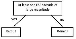
A random forest is a combination of many small decision trees (also known as classification trees). These trees are constructed in unique ways (Friedman et al., 2001). The basic structure of any single decision tree in a random forest begins with a central node and two branches (Rokach & Maimon, 2008, see Figure 10). Then, a tree-building algorithm (we use CART, Breiman et al., 1984/2017) iterates through all variables in the training set to identify one that can split the data as homogeneously as possible. In our case, this involves identifying a variable—typically a saccade magnitude (length)—whose presence indicates belonging to one class, and whose general absence indicates belonging to another class. In short, variables that differentiate between output classes are selected for use in the tree-building process, and variables that do not help differentiate between output classes are not selected, and the CART algorithm determines how to best employ the useful variables. This variable selection process repeats until a stopping criterion—typically a maximum tree depth (in Figure 10, this depth is one) or a minimum node size (number of squares in Figure 10)—is reached. To learn more about decision trees, see, for example, Breiman et al. (1984/2017). Figure 10 shows an example of a possible split in a tree that uses the direction and magnitude of a saccade.
Figure 10. Example of a decision tree. ESE means east-south-east direction of the saccade.
The uniqueness of decision trees in a random forest is that each tree is only given access to a random subset of the data sampled with replacement and each split in the tree is only given access to a random subset of the variables. That is, each tree only uses a random sample of participants’ data—with the possibility of sampling the same participant’s data multiple times—and each split in the tree uses a small subset of the total number of variables. The exact size of each sample is part of the tuning process and our final values can be seen in the supplementary R-code (Dataset5). Allowing each tree to be built on only a subset of data and variables typically leads to a worse-performing tree than if all data were available (Dzeroski & Zenko, 2004). However, the risk of building one (the best) tree only, is that this tree might work perfectly for exactly the given data set, but not on data sets that are similar but slightly different. This is called overfitting. Building many trees using independently sampled data and variables stops any individual tree from drastically overfitting the training data and leads to trees that are relatively uncorrelated (Hansen & Salamon, 1990). These uncorrelated trees are then used together in an ensemble to make classifications, known as the random forest. Each tree predicts the class of the given data—in our case whether the user is seeing the item for the first or second time—and then the votes are totaled. Whichever class receives the most votes is the resulting classification of the random forest (Breiman, 2001).
This technique of simultaneously combining multiple machine learning algorithms—the trees in a random forest—together is known as ensemble learning. This approach is effective since the combined knowledge of many algorithms is often more accurate than any single algorithm (Dzeroski & Zenko, 2004). Here, we train our ensemble using gaze data as inputs and a binary output indicating whether the user is seeing the item for the first time or the second time. We use the randomForest package in R (Liaw & Wiener, 2002) to implement our random forest. Our final, fully-tuned model utilized the following hyperparameters: 1,000 trees, 5 variables considered at each split, a minimum node size of 1, and a maximum tree depth of 5. We identified these optimal hyperparameters using a grid search of size 3^5 (we tried all combinations of three different values for each hyperparameter). Our nested resampling scheme utilized both an outer resampling and an inner resampling of 5-fold cross-validation. The reported best hyperparameters are the average values used across each of our outer resamplings. We likewise evaluated our model using 5-fold cross-validation. To ensure no students’ data were part of both the training and testing data when evaluating our model, we split the data into five groups, each group containing 10 students. We then used the 10 students’ data (yielding a total of 20 student-item pairings) as testing data, and trained our random forest on the remaining 40 students’ data (80 student-item pairings). This process was repeated five times until all students’ data have been separately used as training and testing data. The software used for this data analysis is RStudio (RRID:SCR_000432; SciCrunch Registry). The full reproducible code to build our random forest as used in RStudio as well as the processed data are available through a data repository (Dataset 5). The original data can be found in Dataset 1.
3.4.2 A failed MLA—Using Dwell Time on AOIs
As described at the beginning of section 3.4, we first plotted the data before we analyzed it with an MLA. This plotting is considered part of the data analysis, as the plots can provide indications of what features might be relevant as inputs for the MLA. Differences in where and how long participants looked—fixated—were explored over time throughout each of the four items of interest. As an example, figure 11 shows the fixations for two selected, archetypical participants, L01 and L05, who progressed very differently through the same item (here, the double-histogram Item11). The x-axis, time, has been rescaled from 0 to 1 so fixations could be compared between participants who spent different amounts of time on each item. A time of 0.5, for example, indicates the time at which the given participant is halfway through completing Item11. In this figure, points are jittered (shifted a slight amount in a random direction) to better display the density of points in a given AOI at a given time.
Participant L01, like many participants, fixated on several different AOIs throughout their time working on Item11, often moving back and forth between the graphing area and the corresponding axis. Participant L05, however, spent most of their time fixating on the graph area of both the left and right graphs—stopping briefly to look at the right graph’s vertical axis and label after having spent a considerable amount of time looking at the graphing area. In addition to these two main archetypes, the remaining gaze patterns varied widely between each of the four items and between participants on a given item.
To quantify the differences between student approaches to the before and after items, we began by identifying features (variables) for training our series of random forest models. If the random forest algorithm can consistently differentiate between gaze data from the before and after item in each pairing, then some combination of features must exist that is more prevalent in one item when compared to the other, indicating a difference in gaze patterns between the paired items.
For each of the two item pairings (pairing Item02 and Item20, pairing Item11 and Item21), we began by treating each participant-item combination as our unit of observation, yielding a total of 200 data points (50 participants’ gaze patterns across two items in each of two pairings). For each data point, we calculated the proportional time spent in each AOI. We identified the path each participant took through the AOIs and converted this information into features for our random forest model.
Figure 11. Distribution of gazes of participants L01(left) and L05 (right) over AOIs for Item11.
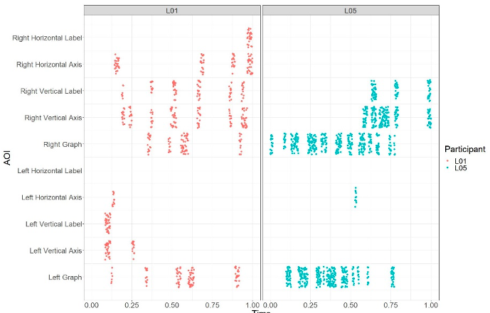
Note. The horizontal axis shows time, which is rescaled from 0 to 1 for each participant individually.
In short, this initial approach was unsuccessful. To prevent readers from scrolling back and forth, we provide a short description of these results here. There were no discernable differences at the individual level between each pairing of before and after items. Participants spent roughly the same proportion of time looking at each of the AOIs when they saw the before items as when they saw the corresponding after item. Though the order in which participants progressed through each of the AOIs differed between before and after items, no discernable pattern emerged, and the correspondingly trained random forest algorithms were unable to accurately predict whether a participant was viewing a before item or an after item in a given pairing. We, therefore, do not further elaborate on this approach in the Results section.
3.4.3 A Successful Approach—Exploring Saccade Direction and Magnitude
Based on previous qualitative work (Boels, Bakker, et al., 2022) we then used directional movements—saccades—first by, again, visually investigating whether differences appeared in saccade patterns between before items and after items. We noticed a clear difference in the pattern of saccades due to the mirrored orientation of the otherwise-identical graphs in Item11 and Item21. Thus, our subsequent analysis focused on mirrored versions of the after items, Item21 and Item20, so that the graph area is made identical to their before counterparts. In other words, we took the gaze coordinates for the mirrored after items and adjusted them to match the corresponding coordinate of the unmirrored before items. Without this un-mirroring, the random forest algorithm could have easily differentiated between gaze data from the before and after items in each pair. Figure 12 shows the patterns of saccades for the same two selected archetypical participants—L01 and L05—on one particular pairing, Item11 and mirrored-Item21. In this figure, all saccades are centered at the origin and radiate outward based on the direction and magnitude of the saccade. Only saccades of magnitudes greater than 200 pixels are shown since these are the saccades used in our final model. Saccades of less than 200 pixels were generally eye movements that are not indicative of students moving from one fixation point to another.
Given the size of the graph areas (width 489 pixels, height 313 pixels for double graph items, 600 x 335 for single graph items), the maximum possible saccade magnitude is 687 pixels (diagonal). The maximum speed for human saccades is approximately 700 degrees per second (Fuchs, 1967; Oohira et al., 1981) which is 570 pixels per 16.7 ms (a sampling rate of 60 Hz equals to one sample every 16.7 ms). Therefore, the maximum for long saccades was set at 600 pixels; longer saccades were considered to be artifacts. Furthermore, we removed ‘saccades’ smaller than 50 pixels. Given the accuracy of the eye tracker (mean 13.4 pixels in the center of the screen and mean 56.6 pixels over all measures), we consider these small ‘saccades’ part of fixations or noise. Although this meant removing more than ninety percent of the measurements on the graph area, the accuracy of our MLA became slightly better.
We defined the beginning of a saccade to be a movement with a velocity greater than 50 pixels per 16.7ms. We defined the end of the saccade as any two consecutive 16.7ms windows where the participant’s gaze had not moved more than 50 pixels. Points of fixation were determined by averaging the x- and y-pixel values of gazes in between two saccades, and each saccade’s direction and magnitude were calculated between these points of fixation.
Figure 12. Saccades of magnitude 200 pixels or more of participants L01 and L05.
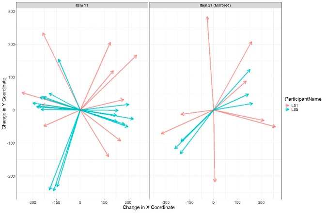
Note. Students’ saccades on the graph area only after mirroring. The number of medium and long saccades decreased from Item11 to Item21 for these two participants. All saccades are shifted to the origin.
Figure 13 shows all saccades of a magnitude of 200 pixels or more for each of the four items. There is a discernable difference in the number of vertically oriented saccades between before and after items, especially in the Item02 and Item20 pairing. The Item11 and Item21 pairing also shows differences in the orientations of many horizontally facing saccades. Notably, there are several more northwest- and southeast-facing saccades in Item11 and more northeast and southwest-facing saccades in Item21 (after mirroring).
We examine differences in students’ gaze patterns on histogram items. If the random forest algorithm can consistently differentiate between gaze data from the before and after item in each pairing, then there must be some combination of features (variables) that is more prevalent in one item when compared to the other, indicating a difference in gaze patterns between the paired items. To construct our random forest model, we tried different sets of features—placing each saccade into mutually exclusive bins depending on the direction, magnitude, and phase of the saccade, regardless of the point of origin. We tested two different directional schemes, two magnitude schemes, and three phase adjustment schemes, yielding a total of twelve combinations. Here, a phase adjustment is an angle (in radians) at which the direction bins are shifted, where 0 radians is equivalent to 0 degrees in mathematics—a saccade pointed eastward—and pi radians is equivalent to 180 degrees—a saccade pointed westward. Table 2 shows the details of each scheme. The direction of each saccade (with no phase shift) was linked to a specific compass rose direction (Figure 14). The direction ESE, for example, aligns with the direction [7π/4, 2π).
Figure 13. Saccades of magnitude 200 pixels or more of all participants on Item11 and Item21 (double-histograms, top) as well as Item02 and Item20 (single-histogram, bottom).
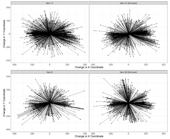
Note. Notice the difference in the density of students’ saccade directions between the before items (left) and after items (right).
We calculated accuracy, sensitivity, and specificity for each combination, seeding our random forest algorithm to obtain reproducible results. We treated the before items as the positive case, meaning that accuracy is defined as the total proportion of times the algorithm correctly identified whether the given data point belonged to the before item or the after item in the pairing. Sensitivity is the proportion of the data points the model identified as belonging to the before item that actually belonged to the before item. Specificity is the proportion of after-item data points that were correctly identified as belonging to the after item. Each metric was calculated using 5-fold cross-validation.
We categorized the features into bins (see Table 2) for two reasons. First, we wanted to extract the variable importance metrics from our random forest in a way that might better inform us why the model was differentiating so well. More specifically, we wanted to know which direction or magnitude of a saccade is more present in one item’s data and not the other’s. If we would have used continuous features, this interpretation would have been much more convoluted to human beings. Second, we also tried a continuous features model. That model performed worse. This might be because saccades that are close in direction and magnitude are functionally identical. In other words, perhaps a saccade of 25 degrees and a saccade of 5 degrees both imply that a student is scanning from left to right, and the difference in angles is either an artifact of data error or a meaningless difference between fixation points.
Table 2
Bins that are used to categorize each saccade for use in our MLA
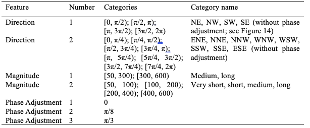
Note. For each feature (variable) the specific categories are indicated by a number. In total, there are two times two times three equals twelve possible combinations.
Our overall research question is: In what way do secondary school students’ histogram interpretations change after solving dotplot items? In this section, we answer this question by answering the following three sub-questions:
The first sub-question is answered by using a random forest model. The twelve combinations of direction, magnitude, and phase schemes (Table 2) yielded accuracies, sensitivities, and specificities that varied between 55% and 88% (Table 3). The standard deviations for each performance metric are reported in parenthesis using 100 resamples. The most accurate combination for both pairings was direction 2, magnitude 2, and phase adjustment 1, which corresponded to the most granular direction and magnitude bins and no phase adjustment. The details of each combination can be seen in Table 2. This best combination yielded a remarkably high 77% accuracy for the single-histogram items (Table 3) and 86% accuracy for the double-histogram items (Table 4). We note that accuracy alone can be potentially misleading—in our study attributing scanpath patterns randomly would yield 50% accuracy. Therefore, an accuracy near 75% is considered good in this low-stake situation, since it would show gains in accuracy well above random guessing. In addition, accuracy needs to be judged together with sensitivity and specificity for which values near 75% are also considered good. Note that this performance may increase if we were to exclude some students for whom we had sparse data for a specific item (e.g., due to data loss for that specific item).
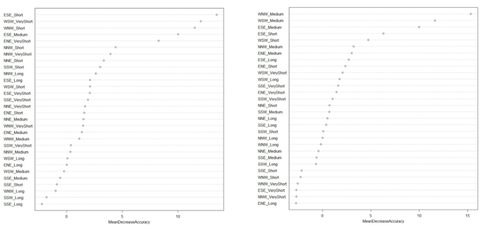
To better understand which features were driving the accuracy of these models, we calculated the importance of each variable (Figure 15) for the best models for each pairing. These plots show the estimated average decrease in accuracy if the given feature was removed from the data set completely. For example, if the number of ESE short saccades was unknown to the random forest, the model for the single-histogram item would see a 15% decrease in absolute accuracy. These metrics are calculated using out-of-bag error estimates (a boot-strapping method for measuring the prediction error for the random forest where a variable is left out of the resampling ‘bag’). The ESE, WNW, and WSW saccades were most important to both models’ accuracies, all being almost horizontal saccades. Almost vertical saccades (e.g., NNW) were less important.
Table 3
Model efficacy on Item02 versus Item20 (single-histogram items)
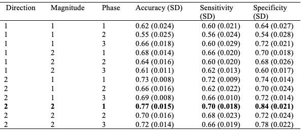
Note. SD = Standard deviation
Table 4
Model efficacy on Item11 versus Item21 (double-histogram items)
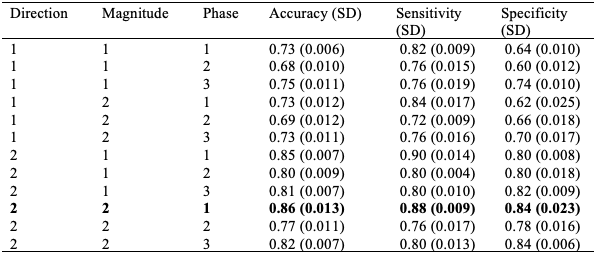
Note. SD = Standard deviation
Figure 14. Compass rose.

Phase 1—no phase adjustment—yielded the best model on average. Direction and magnitude had moderate effects, with more refined bins yielding better-performing models. Both pairings showed a wider variation in accuracies, with low accuracy for more broad categorization schemes and remarkably high accuracy for more refined categorization schemes.
Figure 15. Plots showing the importance of variables for single-histogram MLA-model (left) and double-histogram MLA-model (right).
The machine learning analysis indicated that there are differences in the gazes of students. To investigate whether these changes reflect a change in students’ approaches, we analyzed students’ stimulated recall verbal reports (see Dataset1 for the items). Through qualitative coding of the excerpts of these verbal reports, we answer the second sub-question: What indications can be found in the verbalizations during stimulated recall that changes in students’ approaches to histograms occurred?
Some students learned from the sequence of items, as we can see for example from the transcript of studentL20 for single-histogram Item02:
L20: I think I did 18+8+5∙2+2∙4. And then divided all that by nine. […]
R1: And then you first came up with nine kilos and later you changed it to six kilos. […]
L20: It is not right.
R1: And why is it not right?
L20: It must be somewhere near the three.
R1: Why?
L20: Because there’s a lot less than one kilogram, and relatively a lot two kilograms. And then after that, it really expands to nine kilograms but those are all very small numbers. So, then you end up with three.
R1: Yes. So now that you look at it again you think: I should have given a completely different answer?
L20: Yes.
What this transcript also shows is that this understanding of how to estimate the mean from a histogram took place sometime after single-histogram Item02, but it is not clear when exactly this understanding occurred. For some students, it occurred after (at least one item of) the second series of histogram items, as the following student excerpt shows. This student reflects on the chosen approach in (left-skewed, single histogram) Item19 in the stimulated recall:
L01: The mean will be about between five and nine because there are a lot of values [measured weights] there. And then around seven because that’s a little bit more to the left to zero from the middle between five and nine.
R1: Would you like to look at your eye movements again?
[L01 looks back eye movements]
R1: […] You gave the answer ten. And that’s where you looked.
L01: Ten? [sounds astonished]
R1: Yes, look at your eye movements again.
[L01 looks back eye movements]
L01: Oh yes, in that case, I misread the axes.
For twenty-six students, there was (almost) no room for improvement because they already gave answers within or close to the answer range during the before sequence of single-histogram items. Another four to twelve students seem to have learned specifically from the dotplot items. For example, studentL16 answered seven (instead of 2.7) for single-histogram Item02 but starts giving answers within or very close to the answer range for all following single dotplot items, and continues with these correct answers for the second series of single-histogram items after the dotplot items. During the recall, this student first describes a correct strategy for finding the mean from Item02 which is not in line with the given answer:
L16: Yes, again looking at frequency and weight, and then we see that the one occurred very often and the further you get [to the right] actually the less [frequency]. So, then the mean goes much more to the one than to the high numbers.
R1: Yes, you then said about seven.
L16: Yes, then I looked at it wrong again. Then I got weight and frequency flipped again.
At first glance, there seems to be no real difference in answer correctness between Item02 and Item20 (Table 5). Nevertheless, there are two indications in students’ answers that students learned between Item02 and Item20. First, the answer range chosen for correct answers impacts answer correctness and was set the same for all items. In this study, students seem to prefer whole and half numbers. Enlarging the answer range to include the next whole or half numbers would result in (a non-significant) improvement in answer correctness (see note Table 5). Answer correctness is, therefore, quite sensitive to researchers’ choices. Hence, changes in students’ answers are a better indicator of students’ learning potential.
Second, differences between students’ answers and the actual mean are much lower for Item20 compared to Item02. We calculated the difference between the actual mean and the estimated mean (= Mdiff). Mdiff is, as expected, lower for the after item. We explored if this difference was significant through a one-tailed paired-t-test, as we expected that dotplot items would support students in correctly estimating the mean from histograms in the after items. The assumptions for a paired t-test, such as the unimodality and rough symmetry of the paired differences, were checked and met. The results for before Item02 (Mdiff = 1.1, SD = 1.8) compared to after Item20 (Mdiff = 0.4, SD = 1.7) indicate that it is possible that dotplots improve students’ performance on the after Item, t(49)= -1.7, p = 0.0469 < 0.05. We consider this (and the next) p-value significant in the way the statistician Fisher intended: “in the old-fashioned sense: worthy of a second look” (Nuzzo, 2014, pp. 150–151). The 95%-confidence interval for the differences in Mdiff is <-Inf, ¬¬-0.014] and Cohen’s d measure for effect size is 0.40. Altogether, this points toward an improvement in answers. Note that, on the one hand, effect sizes tend to be larger in researcher-made tests compared to general (standardized) tests as well as in studies with small sample sizes. On the other hand, (very) short interventions often have lower effect sizes (e.g., Bakker et al., 2019). Furthermore, although students’ answers’ correctness improved for the double-histogram item after the dotplot items, this improvement is not significant, as p = 0.3428 > 0.05 (e.g., McNemar, 1947).
Table 5
Answers that are given by the students, N = 50
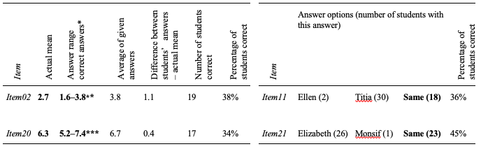
Note. *Experts were also asked to answer these items. Based on these results as well as students’ preference for whole numbers, the answer range was set to +/-1.1 for all items. **If answers 1.5 and 4 had been included, 27 students (54%) would have answered correctly. ***If answers 5 and 7.5 had been included, 31 students (62%) would have answered correctly. Correct answers are in bold.
Instead of attributing the smaller Mdiff —for single histogram items–—to the solving of dotplot items, one alternative explanation is that the mean of Item20 (M = 6.3) compared to Item02 (M = 2.7) is closer to the mean of the frequencies (M = 4.9 for both). Nevertheless, we do not expect that this is the case, as for another left skewed item of this sequence of items (Item06, not further reported here, see Boels, Garcia Moreno-Esteva, et al., accepted) the mean of the frequencies (M = 7.1) was also close to the mean of this item (M = 5.7), but the difference between actual and students’ mean (Mdiff = 1.2) was similar to before Item02. To further exclude this alternative explanation, we suggest enlarging the difference between the actual mean and the mean of frequencies by adding more data (e.g., 50 packages) to the graphs. This number of added packages should not be too high to avoid students guessing from the size of the numbers what the weights are, as may have played a role in an item with SAT scores according to Kaplan et al. (2014).
In this study, we answer the main research question of in what way secondary school students’ histogram interpretations change after solving dotplot items. More specifically, we look at students’ estimations and comparisons of means from histograms. We expected that solving dotplot items would focus students’ attention on the measured variable (weight) being depicted along the horizontal axis. In turn, that would invite students to estimate the mean of the weights (along the horizontal axis) instead of the mean of the frequencies (along the vertical axis) in the histograms. We examined three indications that taken together can suggest detailed-level changes in students’ histograms interpretations: a change in students’ gaze patterns, a shift in students’ strategy for solving the histogram items, and an improvement in students’ answers. If the changes are for the better, the relevance of knowing them is that they could underpin the learning potential of using dotplot items before solving histogram items—a hypothesis put forward by researchers in statistics education.
For the first indicator—a change in students’ eye movements—we looked at differences in students’ gaze or scanpath patterns on the graph area through a machine learning algorithm. Two main differences—on the student level—between scanpath patterns on before and after items were found. First, there were proportionally fewer horizontal directions (ESE/WNW) in the gaze patterns on the after items than on the before items. Second, proportionally more vertical directions (NNW/NNE) were found in the after items. A horizontal gaze pattern is associated with an incorrect strategy while a vertical gaze pattern is associated with a correct strategy. Our best implementations of random forests were able to accurately classify (roughly 80% of the instances) whether it was the first (before) or second (after) time a participant had seen an item in one of two pairings. What we can attest to, is a significant, discernable difference in the way participants looked at the before items and when viewing the mirrored after versions, even after accounting for mirroring in the graphs. As we could not identify other confounding factors, it seems reasonable to conclude that our findings exhibit evidence that students changed the way they approached an item when seeing its mirrored version later in this sequence of items. The results of our MLA are in line with the results of previous studies (Boels, Bakker, et al., 2022; Boels, Garcia Moreno-Esteva, et al., accepted).
We cannot be certain whether the observed differences in gazes indicate a change in strategies. Although scanpaths can disclose students’ strategies at a detailed level, the relationship between eye movements and strategies is task-dependent (e.g., Orquin & Holmqvist, 2017; Russo, 2010). In addition, not every eye movement is part of a task-specific strategy (e.g., Schindler & Lilienthal, 2019). Therefore, other data—such as our second and third indicators—are often needed to support or refute conjectures about the association between scanpath patterns and strategies.
The second indicator of changes in students’ histograms interpretations—a shift in students’ strategy for solving the items—was evaluated by coding students’ stimulated recall verbal reports. The excerpts provide evidence that at least some students changed their strategies, from an incorrect approach for estimating and comparing means from histograms to a correct approach, during or after solving the dotplot items.
The third indicator—improvement in students’ answers—was explored through both answer correctness, the difference between students’ estimation of the mean and the actual mean for single-histogram items, and the changes in students’ answers on the double-histogram multiple-choice items. Answer correctness did not change significantly on either item type. Nevertheless, the difference in students’ estimation of the mean compared to the actual mean was significantly smaller for the after item compared to the before item. We use ‘significantly’ here in the sense Fisher intended: worthy of further investigation. Data collection with new and more participants—from the same population (Dutch Grades 10–12 pre-university track students)—is needed to investigate the hypothesis that this difference becomes smaller, that there is a change in multiple-choice answers, and that both are due to solving the dotplot items.
The three indicators taken together suggest that at least some students changed their strategy during or after solving the sequence of dotplot items. A change in gaze behavior was observable through our machine learning analysis with random forests. Depending on how learning is defined, this change could point to a learning effect of solving dotplot items.
Interpreting the results, we abductively arrived at the following explanations for our results. First, the change toward proportionally more vertical gazes on the after items is in line with the conjecture that the absence of a vertical scale in dotplots can turn students’ attention toward the horizontal scale which is where the variable is presented in both histograms and dotplots. These students possibly figured out that the mean can be estimated from the measured values along the horizontal axis. However, we cannot rule out that factors other than solving dotplot items could have contributed to this change.
Second, we consider the most likely explanation for the mixed results that solving dotplot items promoted readiness for learning (Church & Goldin-Meadow, 1986) about histograms. Having students reflect on their previous strategy while they were cued with their own gazes during retrospective verbal reporting then might have given them new insights. After solving the dotplot items, histogram items seem to lie within the region of sensitivity for learning, hence within students’ zone of proximal development (Vygotsky, 1978). It is possible that the questions asked by the researcher (an adult), which were intended to figure out how students solved the items, unintentionally stimulated students’ thinking by asking them to explain—hence, reflect on—their strategies. Further research is needed to check this explanation. An alternative explanation for the results would be that other items after the second series of histogram items induced students’ thinking. Although we cannot exclude this alternative, we regard this to be less likely.
Further discussing the results, we note that this study is novel in the following ways. First, to the best of our knowledge, our study is the first in education that combined a quantitative analysis of the scanpath patterns found in spatial gaze data with insights from a previous qualitative study about what part of the scanpath pattern is relevant for students’ strategies (namely, the scanpath on the graph area only). The use of qualitative insights contributes to the validity of the study while the quantitative approach through machine learning analysis contributes to the reliability of it. Most eye-tracking studies that use spatial measures investigate the sequence of AOIs (Garcia Moreno-Esteva et al., 2020) and the same holds for those combining it with MLAs (e.g., Garcia Moreno-Esteva et al., 2018). Instead, we used vectors (i.e., direction and magnitude) of saccades. Studies in education that utilize vectors are rare (e.g., Dewhurst et al., 2018). Second, novel is the use of an MLA for finding differences in gazes that are relevant to changes in students’ task-specific strategies between tasks.
Our study has several limiting factors. First, many of the participants’ gaze data contained data loss. Although data loss is normal due to blinking or looking away from the screen, some data loss could be avoided by pre-excluding participants who wear glasses, contact lenses, or mascara. In addition, an eye tracker could be used that is better in catching gazes from people with epicanthic folds (almond eyes). As we aimed for a naturalistic setting, we did not exclude any of such participants. In addition, for some participants, we had sparse data. Some of these participants spent only a few seconds looking at a given item. This made predictions and training more challenging. Most of these participants appeared to parse the graph and answer the corresponding question(s) in a rapid but reasonable manner, although one participant appeared to scan the graph and answer the question in such a rapid way that it is unlikely that they had time to fully understand what the graph was depicting. Since no participants’ data were removed, some amount of data cleaning and removal of outlier participants would likely increase the accuracy of our random forests, although our data collection scheme does not allow us to know with certainty why a certain participant’s gaze data were sparse for a particular item.
A second limiting factor was that we restricted our final analysis to the graph area of each item, excluding AOIs such as the axes labels and the graph title. The inclusion of these AOIs yielded more noise and worse results, but further work might investigate the possibility of productively including them. Third, answer correctness and students’ strategies correspond only to a limited extent. Finally, and most importantly, our sample size—50 participants and 2 items yielding 100 participant-item-pairings—is relatively small for machine learning and statistical analysis. Our results indicate strong evidence of a change in gaze patterns between the before and after items, but more data are needed to generalize these findings appropriately.
A theoretical contribution of this study is that having students solve non-stacked (‘messy’) dotplot items can create readiness for learning histograms. A reflection phase seems to be needed to make use of the knowledge obtained. We speculate that this partly explains the results from the literature on dotplots (e.g., Garfield & Ben-Zvi, 2008; Lyford, 2017). Another reason for these results, we believe, is that only non-stacked dotplots contribute to students’ understanding of where the measured value is. Stacked dotplots already contain an information reduction step (the binning) that could lead to similar misinterpretations as for histograms (see Boels, Bakker, Van Dooren & Drijvers, 2019). We, therefore, advise investigating whether stacked dotplots need to be avoided in secondary education.
As a first methodological implication, our study shows how an MLA in combination with eye-tracking data can be used to reveal phenomena that are of interest to researchers of education. Future use could include interpreting graphical representations in biology, physics, economics, and geography. By choosing features (variables) that are relevant to the phenomena of interest (here: students’ strategies for solving a histogram item) and meaningful to the researchers, an MLA can give insights into subtle, detailed-level differences in students’ strategies that are hard to detect through other research methods, such as time measures in eye-tracking research or qualitative analysis of gaze data by researchers.
A second methodological implication is that there seems to be a practice effect within a sequence of items for at least some students, in line with suggestions from Lumsden (1976). A practice effect refers to improved performance after ‘practicing’ (i.e., repeatedly solving similar or the same items). This is also important for judging the validity of summative assessments. More research is needed to confirm this within-a-test practice effect. Catron (1978) found an effect of item types on an IQ test. For example, he showed that the development of a strategy in strategic items improved performance on retesting. The present study does not consider an effect of item type. Further research is needed to find out whether and for what items the order and type of items influence the within-a-test practice effect.
What are the possible implications of our findings? The ML approach is generalizable to other sequences of items or any instance when a user may wish to classify eye-tracking data into one of many discrete categories. Further analysis is needed to correlate the number of saccades of specific directions and magnitudes with particular viewing strategies. In other words, does the presence of certain features (variables, such as horizontal or vertical saccades) indicate students taking a particular strategy, and if so, is this strategy more common when viewing a before item as opposed to an after item? Moreover, we think our ML approach can also be used when researchers want to know whether solving X (a question about a graph or image) changes the way students solve Y (a question about a different type of graph or image).
For testing a future hypothesis that students’ estimations of the mean from histograms become closer to the actual mean after solving dotplot items, we suggest making a sequence of 24 items: eight histogram items (improved versions of the existing items from the original sequence with more data in them as well as one extra left skewed single histogram and one extra double histogram), eight dotplot items (all items containing the same data as the first eight histograms) and then again eight histogram items (all mirrored versions of the first eight histogram items). To check a future hypothesis that giving students stacked dotplots is a less effective way to scaffold them, a variant of this design could be made with stacked dotplots only, instead of non-stacked dotplots (with the stacks in between two values on the horizontal scale; all stacked dotplots contain the same data as the first eight histograms). To check a future hypothesis that the reflection phase is important, a variant with and without stimulated recall verbal reports could be conducted followed by another series of histogram items. In all these variants, machine learning analysis can support this hypothesis testing.
For practitioners, insight into what students learn from doing a sequence of items is also relevant for homework and formative assessment, in particular, if no feedback is given—which is quite a common situation (e.g., when there is less student-teacher interaction). The observed differences in gaze patterns together with the other evidence in this study, suggest that a sequence of items can create readiness for learning, but a teacher may still be needed to ensure that students reach their full potential.
This research is funded with a Doctoral Grant for Teachers from the Dutch Research Council (NWO), number 023.007.023 awarded to Lonneke Boels. Any opinions, findings, or recommendations expressed in this material are those of the authors and do not necessarily reflect the views of the Dutch Research Council. We thank the following people for their contributions to this study. Nathalie Kuijpers for checking the document on style and English, Ciera Lamb for proofreading a previous version for American English, Anna Shvarts for assisting during the last day of data collection, Wim Van Dooren for his contribution to the design of the eye-tracking study, Rutmer Ebbes for his contribution to the pilot eye-tracking study (Boels et al., 2018), Aline Boels for the programming of the HTML-files containing the items, Juri Boels for transcribing almost all verbal reports, Iljo Boels for exporting gaze plots and heatmaps, Willem den Boer for writing the macros for processing the eye-tracking data. Furthermore, LB thanks all the people organizing and contributing to the eye-tracking seminars of the UU, especially Ellen Kok, Margot van Wermeskerken, Roy Hessels, Ignace Hooge, and Jos Jaspers. LB also thanks the Faculty of Social and Behavioral Sciences for lending the laptop and Tobii-XII-60 eye tracker for this research.
The authors declare that there is no potential conflict of interest.
The datasets analyzed for this study can be found in the DataVerseNL repository.
Dataset1: https://doi.org/10.34894/WEKAYE
Dataset3: https://doi.org/10.34894/7KNEOH
Dataset5: https://doi.org/10.34894/PLCEBC
AB, PD, and LB contributed to the conception and design of the study. The data were collected and cleaned by LB. ML analysis and statistical tests were conducted by AL. LB wrote the first draft of the introduction, materials and methods, and results section except for most of the texts on the ML analysis and results. The latter was initially written by AL. Results and Discussion were initially written by LB and AL. All authors contributed to manuscript revision, and finally read and approved the submitted version.
Allmond, S. & Makar, K. (2014). From hat plots to box plots in TinkerPlots: Supporting students to write conclusions which account for variability in data. In K. Makar, B. de Sousa, & R. Gould (Eds.), Sustainability in statistics education. Proceedings of the Ninth International Conference on Teaching Statistics . https://iase-web.org/icots/9/proceedings/pdfs/ICOTS9_2E1_ALLMOND.pdf?1405041584
Bakker, A. (2004a). Design research in statistics education: On symbolizing and computer tools [Doctoral dissertation, Utrecht University]. https://dspace.library.uu.nl/handle/1874/893
Bakker, A. (2004b). Reasoning about shape as a pattern in variability. Statistics Education Research Journal, 3 (2), 64–83. http://iase-web.org/documents/SERJ/SERJ3(2)_Bakker.pdf?1402525004
Bakker, A., Biehler, R., & Konold, C. (2004). Should young students learn about box plots? In G. Burrill & M. Camden (Eds.), Curricular development in Statistics Education: International Association for Statistical Education 2004 Roundtable, (pp. 163–173). International Statistical Institute. https://iase-web.org/documents/papers/rt2004/4.2_Bakker_etal.pdf?1402524988
Bakker, A., Cai, J., English, L. Kaiser, G., Mesa, V., & Van Dooren, W. (2019). Beyond small, medium, or large: Points of consideration when interpreting effect sizes. Educational Studies in Mathematics, 102, 1–8. https://doi.org/10.1007/s10649-019-09908-4
Bargagliotti, A., Franklin, C., Arnold, P., Gould, R., Johnson, S., Perez, L., & Spangler, D. (2020). Pre-K-12 guidelines for assessment and instruction in statistics education (GAISE) report II. American Statistical Association and National Council of Teachers of Mathematics. https://www.amstat.org/asa/files/pdfs/GAISE/GAISEIIPreK-12_Full.pdf
Bennett, R. E. (2011) Formative assessment: A critical review. Assessment in Education: Principles, Policy & Practice, 18 (1), 5–25, https://doi.org/10.1080/0969594X.2010.513678
Ben-Zvi, D. & Garfield, J. (2004). Research on reasoning about variability: A forward. Statistics Education Research Journal, 3(2), 4–6. http://iase-web.org/documents/SERJ/SERJ3(2)_forward.pdf?1402525004
Boels, L., Bakker, A., Van Dooren, W., & Drijvers, P. (2019). Conceptual difficulties when interpreting histograms: A review. Educational Research Review, 28, Article 100291. https://doi.org/10.1016/j.edurev.2019.100291
Boels,L., Bakker, A., & Drijvers, P. (2019). Eye tracking secondary school students’ strategies when interpreting statistical graphs. In M. Graven, H. Venkat, A.A. Essien, & P. Vale (Eds.), Proceedings of the Forty-third Conference of the International Group for the Psychology of Mathematics Education, 2, (pp. 113–120). https://www.igpme.org/publications/current-proceedings/
Boels, L., Bakker, A., Van Dooren, W., & Drijvers, P. (2022). Secondary school students’ strategies when interpreting histograms and case-value plots: an eye-tracking study . [Manuscript submitted for publication] Freudenthal Institute, Utrecht University.
Boels, L., Ebbes, R. Bakker, A., Van Dooren, W., & Drijvers, P. (2018). Revealing conceptual difficulties when interpreting histograms: An eye-tracking study. Invited paper, refereed. In M. A. Sorto, A. White, & L. Guyot (Eds.), Looking back, looking forward. Proceedings of the Tenth International Conference on Teaching Statistics, (pp. 1–4). https://iase-web.org/icots/10/proceedings/pdfs/ICOTS10_8E2.pdf
Boels, L., Garcia Moreno-Esteva, E., Bakker, A., & Drijvers, P. (accepted). Automated gaze-based identification of students’ strategies in histogram tasks through an interpretable model and a machine learning algorithm. International Journal of Artificial Intelligence in Education.
Breiman, L., Friedman, J. H., Olshen, R. A., & Stone, C. J. (2017). Classification and regression trees. Routledge. (Original work published 1984) https://doi.org/10.1201/9781315139470
Breiman, L. (2001). Random forests. Machine learning, 45(1), 5–32. https://doi.org/10.1023/A:1010933404324
Capraro, M. M., Kulm, G., & Capraro, R. M. (2005). Middle grades: Misconceptions in statistical thinking. School Science & Mathematics, 105(4), 165–174. https://doi.org/10.1111/j.1949-8594.2005.tb18156.x
Catron, D. W. (1978). Immediate test-retest changes in WAIS scores among college males. Psychological Reports, 43(1), 279–290. https://doi.org/10.2466/pr0.1978.43.1.279
Church, R.B., & Goldin-Meadow, S. (1986). The mismatch between gesture and speech as an index of transitional knowledge. Cognition, 23 (1), 43–71. https://doi.org/10.1016/0010-0277(86)90053-3
Clayden, A., & Croft, M. (1990). Statistical consultation—who’s the expert? Annals of Mathematics and /Artificial Intelligence, 2 , 65–75. https://doi.org/10.1007/BF01530997
Cohen, S. (1996). Identifying impediments to learning probability and statistics from an assessment of instructional software. Journal of Educational and Behavioral Statistics, 21(1), 35–54. https://doi.org/10.2307/1165254
Cooper, L. L. (2018). Assessing students’ understanding of variability in graphical representations that share the common attribute of bars. Journal of Statistics Education, 26(2), 110–124. https://doi.org/10.1080/10691898.2018.1473060
Cooper, L. L., & Shore, F. S. (2008). Students’ misconceptions in interpreting center and variability of data represented via histograms and stem-and-leaf plots. Journal of Statistics Education,16(2). https://doi.org/10.1080/10691898.2008.11889559
Dabos, M. (2014). A glimpse of two year college instructors’ understanding of variation in histograms. In K. Makar, B. de Sousa, and R. Gould (Eds.). Sustainability in statistics education. Proceedings of the Ninth International Conference on Teaching Statistics (pp. 1–4). https://icots.info/9/proceedings/pdfs/ICOTS9_C150_DABOS.pdf
delMas, R., Garfield, J., & Ooms, A. (2005). Using assessment items to study students’ difficulty reading and interpreting graphical representations of distributions. Proceedings of the fourth international research forum on statistical reasoning, literacy, and reasoning. University of Auckland. https://www.causeweb.org/cause/archive/artist/articles/SRTL4_ARTIST.pdf
delMas, R., & Liu, Y. (2005). Exploring students’ conceptions of the standard deviation. Statistics Education Research Journal,4(1), 55–82. http://iase-web.org/documents/SERJ/SERJ4(1)_delMas_Liu.pdf?1402525005
Dewhurst, R., Foulsham, T., Jarodzka, H., Johansson, R., Holmqvist, K., & Nyström, M. (2018). How task demands influence scanpath similarity in a sequential number-search task. Vision Research, 149, 9–23. https://doi.org/10.1016/j.visres.2018.05.006
Dzeroski, S., & Zenko, B. (2004). Is combining classifiers with stacking better than selecting the best one? Machine Learning,54(3), 255–273. https://doi.org/10.1023/B:MACH.0000015881.36452.6e
Falleti, M. G., Maruff, P., Collie, A. & Darby, D. G. (2006). Practice effects associated with the repeated assessment of cognitive function using the CogState battery at 10-minute, one week and one month test-retest intervals, Journal of Clinical and Experimental Neuropsychology, 28(7), 1095–1112. https://doi.org/10.1080/13803390500205718
Friedman, J., Hastie, T., & Tibshirani, R. (2001). The elements of statistical learning . Springer series in statistics. https://link.springer.com/book/10.1007/978-0-387-21606-5
Fuchs, A. F. (1967). Saccadic and smooth pursuit eye movements in the monkey. The Journal of Physiology, 191(3), 609–631. https://doi.org/10.1113/jphysiol.1967.sp008271
Gal, I. (1995). Statistical tools and statistical literacy: The case of the average. Teaching Statistics, 17(3), 97–99. https://doi.org/10.1111/j.1467-9639.1995.tb00720.x
Gal, I. (2002). Adults’ statistical literacy: Meanings, components, responsibilities. International statistical review, 70(1), 1–25. https://iase-web.org/documents/intstatreview/02.Gal.pdf
Gal, I & Geiger, V. (2022). Welcome to the era of vague news: A study of the demands of statistical and mathematical products in the COVID‑19 pandemic media. Educational Studies in Mathematics, 111,5–28. https://doi.org/10.1007/s10649-022-10151-7
Garcia Moreno-Esteva, E., Kervinen, A., Hannula, M. S., & Uitto, A. (2020). Scanning signatures: A graph theoretical model to represent visual scanning processes and a proof of concept study in biology Education.Education Sciences, 10(5), Article 141. https://doi.org/10.3390/educsci10050141
Garcia Moreno-Esteva, E., White, S. L. J., Wood, J. M., & Black, A. A. (2018). Application of mathematical and machine learning techniques to analyse eye tracking data enabling better understanding of children’s visual cognitive behaviours.Frontline Learning Research, 6(3), 72–84. https://doi.org/10.14786/flr.v6i3.365
Garfield, J. (2002). Histogram sorting. Statistics teaching and resource library (STAR). https://amser.org/index.php?P=AMSER--ResourceFrame&resourceId=8554
Garfield, J. B., & Ben-Zvi, D. (2008). Learning to reason about distribution. In J. Garfield & D. Ben-Zvi (Eds). Developing students’ statistical reasoning: Connecting research and teaching practice (pp. 165–186). Springer. https://link.springer.com/content/pdf/10.1007/978-1-4020-8383-9_8.pdf
Godau, C. Haider, H., Hansen, S., Schubert, T., Frensch, P. A., Gaschler, R. (2014). Spontaneously spotting and applying shortcuts in arithmetic—a primary school perspective on expertise. Frontiers in Psychology – Cognition, 5 , 1664–1078, Article e556. https://doi.org/10.3389/fpsyg.2014.00556
Goldberg, J. H., & Helfman, J. I. (2010). Comparing information graphics: A critical look at eye tracking. Proceedings of the 3rd BELIV’10 Workshop: Beyond time and errors: novel EvaLuation methods for Information Visualization (pp. 71–78). https://doi.org/10.1145/2110192.2110203
Guan, Z., Lee, S., Cuddihy, E., & Ramey, J. (2006). The validity of the stimulated retrospective think-aloud method as measured by eye tracking. Proceedings of the SIGCHI Conference on Human Factors in Computing Systems (pp. 1253–1262). Association for Computing Machinery. https://doi.org/10.1145/1124772.1124961
Guerra-Carrillo, B. C., & Bunge, S.A. (2018). Eye gaze patterns reveal how reasoning skills improve with experience. npj Science of Learning, 3,Article 18. https://doi.org/10.1038/s41539-018-0035-8
Hansen, L. K., & Salamon, P. (1990). Neural network ensembles. IEEE transactions on pattern analysis and machine intelligence, 12, 993–1001. https://doi.org/10.1109/34.58871
Heilbronner, R. L., Sweet, J. J., Attix, D. K., Krull, K. R., Henry, G. K., & Hart, R. P. (2010). Official position of the American Academy of Clinical Neuropsychology on serial neuropsychological assessments: The utility and challenges of repeat test administrations in clinical and forensic contexts, The Clinical Neuropsychologist, 24(8), 1267–1278. https://doi.org/10.1080/13854046.2010.526785
Hessels, R. S., Niehorster, D. C., Nyström, M., Andersson, R., & Hooge, I. T. C. (2018). Is the eye-movement field confused about fixations and saccades? A survey among 124 researchers.Royal Society Open Science, 5(8), 1–23. https://doi.org/10.1098/rsos.180502
Hinton-Bayre, A. D. (2010). Deriving reliable change statistics from test–retest normative data: Comparison of models and mathematical expressions. Archives of Clinical Neuropsychology, 25(3), 244–256. https://doi.org/10.1093/arclin/acq008
Hohn, R. W. (1992). An analysis of the components of curriculum-based assessment [Doctoral dissertation. University of Denver]. https://www.proquest.com/openview/abb4ea5179410900d6e2af9a7473f0e9/1?pq-origsite=gscholar&cbl=18750&diss=y
Holmqvist, K., Örbom, S. L., Hooge, I. T. C., Niehorster, D. C., Alexander, R. G., Andersson, R., Benjamins, J. S., Blignaut, P., Brouwer, A-M., Chuang, L. L., Dalrymple, K. A., Drieghe, D., Dunn, M. J., Ettinger, U., Fiedler, S., Foulsham, T., Van der Geest, J. N., Witzner Hansen, D., Hutton, S., … Hessels, R. S. (2023). Eye tracking: empirical foundations for a minimal reporting guideline. Behavior Research Methods, 55,364–416. https://doi.org/10.3758/s13428-021-01762-8
Hyönä, J. (2010). The use of eye movements in the study of multimedia learning. Learning and Instruction, 20(2), 172–176. https://doi.org/10.1016/j.learninstruc.2009.02.013
James, G., Witten, D., Hastie, T., & Tibshirani, R. (2013). An introduction to statistical learning. Springer texts in statistics, 112. Springer.
Jarodzka, H., Van Gog, T., Dorr, M., Scheiter, K., & Gerjets, P. (2013). Learning to see: Guiding students’ attention via a model’s eye movements fosters learning.Learning and Instruction,25, 62–70. https://doi.org/10.1016/j.learninstruc.2012.11.004
Kaakinen, J.K. (2021). What can eye movements tell us about visual perception processes in classroom contexts? Commentary on a special issue. Educational Psychology Review, 33, 169–179. https://doi.org/10.1007/s10648-020-09573-7
Kaplan, J. J., Gabrosek, J. G., Curtiss, P., & Malone, C. (2014). Investigating student understanding of histograms.Journal of Statistics Education, 22(2), 1–30. https://doi.org/10.1080/10691898.2014.11889701
Khalil, K. A. I. (2005). Expert-novice differences: Visual and verbal responses in a two-group comparison task [Master’s thesis, University of Massachusetts]. https://scholarworks.umass.edu/theses/2428
Konold, C., Higgins, T., Russell, S. J., & Khalil, K. (2015). Data seen through different lenses. Educational Studies in Mathematics,88(3), 305–325. https://doi.org/10.1007/s10649-013-9529-8
Konold, C., & Pollatsek, A. (2002). Data analysis as the search for signals in noisy processes. Journal for Research in Mathematics Education, 33(4), 259–289. https://www.jstor.org/stable/749741
Kragten, M., Admiraal, W., & Rijlaarsdam, G. (2015). Students’ learning activities while studying biological process diagrams.International Journal of Science Education, 37(12), 1915–1937. https://doi.org/10.1080/09500693.2015.1057775
Lai, M., Tsai, M., Yang, F., Hsu, C., Liu, T., Lee, S. W., Lee, M., Chiou, G., Liang, J., & Tsai, C. (2013). A review of using eye-tracking technology in exploring learning from 2000 to 2012.Educational Research Review, 10, 90–115. https://doi.org/10.1016/j.edurev.2013.10.001
Lem, S., Onghena, P., Verschaffel, L., & Van Dooren, W. (2013). On the misinterpretation of histograms and box plots. Educational Psychology, 33 (2), 155–174. https://doi.org/10.1080/01443410.2012.674006
Liaw A, Wiener M (2002). Classification and regression by randomForest. R News, 2(3), 18–22. https://CRAN.R-project.org/doc/Rnews/ .
Lievens, F., Reeve, C. L., & Heggestad, E. D. (2007). An examination of psychometric bias due to retesting on cognitive ability tests in selection settings. Journal of Applied Psychology, 92(6), 1672–1682. https://ink.library.smu.edu.sg/lkcsb_research/5693
Lumsden, J. (1976). Test theory. Annual Review of Psychology, 27 (1), 251–280. https://doi.org/10.1146/annurev.ps.27.020176.001343
Lyford, A. J. (2017). Investigating undergraduate student understanding of graphical displays of quantitative data through machine learning algorithms [Doctoral dissertation, University of Georgia]. https://iase-web.org/documents/dissertations/17.AlexanderLyford.Dissertation.pdf
Lyford, A., & Boels, L. (2022). Using machine learning to understand students’ gaze patterns on graphing tasks. Invited paper: Refereed. In S. A. Peters, L. Zapata-Cardona, F. Bonafini, & A. Fan (Eds.), Bridging the Gap: Empowering & Educating Today’s Learners in Statistics. Proceedings of the Eleventh International Conference on Teaching Statistics (pp. 1–6).ISI/IASE. https://doi.org/10.52041/iase.icots11.T8D2
Lyle, J. (2003). Stimulated recall: A report on its use in naturalistic research. British Educational Research Journal, 29,861–878. https://www.jstor.org/stable/1502138
Makar, K., & Confrey, J. (2004). Secondary teachers’ statistical reasoning in comparing two groups. In D. Ben-Zvi & J. Garfield (Eds.), The challenge of developing statistical literacy, reasoning and thinking (pp. 353–374). Springer. https://rdcu.be/diI3P
McGatha, M., Cobb, P., & McClain, K. (2002). An analysis of students’ initial statistical understandings: Developing a conjectured learning trajectory. The Journal of Mathematical Behavior, 21(3), 339–355. https://doi.org/10.1016/S0732-3123(02)00133-5
McIntyre, N. A., Draycott, B., & Wolff, C. E. (2022). Keeping track of expert teachers: Comparing the affordances of think-aloud elicited by two different video perspectives. Learning and Instruction, 80, Article 101563. https://doi.org/10.1016/j.learninstruc.2021.101563
McNemar, Q. (1947). Note on the sampling error of the difference between correlated proportions or percentages. Psychometrika, 12(2), 153–157. https://doi.org/10.1007/BF02295996
Meletiou, M. (2000). Students’ understanding of variation: An untapped well in statistical reasoning [Doctoral dissertation, University of Texas]. http://iase-web.org/documents/dissertations/00.Meletiou.Dissertation.pdf
Mokros, J., & Russell, S. J. (1995). Children’s concepts of average and representativeness.Journal for Research in Mathematics Education,26(1), 20–39. https://doi.org/10.2307/749226
Nuzzo, R. (2014). Scientific method: Statistical errors. Nature, 506, 150–152. https://doi.org/10.1038/506150a
O’Dell, R.S. (2012). The mean as balance point. Mathematics Teaching in the Middle School, 18(3), 148–155. https://www.jstor.org/stable/10.5951/mathteacmiddscho.18.3.0148
Oohira, A., Okamoto, M., & Ozawa, T. (1981). 正常人の衝動性眼球運動最大速度について [Peak velocity of normal human saccadic eye movements (author’s translation)]. 日限会誌 [Journal of the Japanese Society of Ophthalmology], 85 (11), 2001–2007. https://pubmed.ncbi.nlm.nih.gov/7337121/ or https://www.researchgate.net/publication/15862222_Peak_velocity_of_normal_human_saccadic_eye_movements_author%27s_transl
Orquin, J. L., & Holmqvist, K. (2017). Threats to the validity of eye-movement research in psychology.Behavior Research Methods, 50(4), 1645–1656. https://doi.org/10.3758/s13428-017-0998-z
Płomecka, M.B. Barańczuk-Turska, Z., Pfeiffer, C., & Langer, N. (2020). Aging effects and test–retest reliability of inhibitory control for saccadic eye movements. eNeuro, 7(5). https://doi.org/10.1523/ENEURO.0459-19.2020
Rokach, L., & Maimon, O. (2008). Data mining with decision trees: Theory and applications. Toh Tuck Link: World Scientific. https://doi.org/10.1142/9097
RStudio. SciCrunch Registry. https://posit.co/download/rstudio-desktop/
Russo, J. E. (2010). Eye fixations as a process trace. In M. Schulte-Mecklenbeck, A. Kühberger, and R. Ranyard (Eds.), Handbook of process tracing methods for decision research (pp. 43–64). Psychology Press. https://www.researchgate.net/publication/285189001_Eye_fixations_as_a_process_trace
Scharfen, J., Jansen, K. & Holling, H. (2018). Retest effects in working memory capacity tests: A meta-analysis. Psychonomic Bulletin & Review, 25,2175–2199. https://doi.org/10.3758/s13423-018-1461-6
Schindler, M., & Lilienthal, A. J. (2019). Domain-specific interpretation of eye-tracking data: Towards a refined use of the eye-mind hypothesis for the field of geometry.Educational Studies in Mathematics, 101, 123–139. https://doi.org/10.1007/s10649-019-9878-z
Setiawan, E. P., & Sukoco, H. (2021). Exploring first year university students’ statistical literacy: A case on describing and visualizing data. Journal on Mathematics Education, 12(3), 427–448. https://ejournal.unsri.ac.id/index.php/jme/article/view/13202
Strohmaier, A. R., MacKay, K. J., Obersteiner, A., & Reiss, K. M. (2020). Eye-tracking methodology in mathematics education research: A systematic literature review.Educational Studies in Mathematics, 104, 147–200. https://doi.org/10.1007/s10649-020-09948-1
Temkin, N. R., Heaton, R. K., Grant, I., & Dikmen, S. S. (1999). Detecting significant change in neuropsychological test performance: a comparison of four models. Journal of the International Neuropsychological Society, 5(4), 357–369. https://doi.org/10.1017/s1355617799544068
Tiefenbruck, B. F. (2007). Elementary teachers conceptions of graphical representations of categorical data [Doctoral dissertation. University of Minnesota]. https://conservancy.umn.edu/handle/11299/91699
Tobii (n.d.). Tobii Studio. Users’ Manual. Version 3.4.5. https://www.tobiipro.com/siteassets/tobii-pro/user-manuals/tobii-pro-studio-user-manual.pdf/?v=3.4.5
Van Gog, T., & Jarodzka, H. (2013). Eye tracking as a tool to study and enhance cognitive and metacognitive processes in computer-based learning environments. In R. Azevedo, and V. Aleven (Eds.), International handbook of metacognition and learning technologies (pp. 143–156). Springer. https://doi.org/10.1007/978-1-4419-5546-3_10
Van Gog, T., Paas, F., Van Merriënboer, J. J., & Witte, P. (2005). Uncovering the problem-solving process: Cued retrospective reporting versus concurrent and retrospective reporting.Journal of Experimental Psychology: Applied, 11(4), 237–244. https://doi.org/10.1037/1076-898X.11.4.237
Vygotsky, L. S. (1978). Mind in society: The development of higher psychological processes. Harvard University Press. https://www.hup.harvard.edu/catalog.php?isbn=9780674576292