
Frontline Learning Research Vol.14 No. 1 (2026) 1
- 37
ISSN 2295-3159
1iXperium Centre of Expertise
Learning with ICT, HAN University of Applied Sciences, Nijmegen,
The Netherlands
2National Education Lab AI, Radboud University,
Nijmegen, The Netherlands
3Department of Education and Pedagogy, Utrecht
University, Utrecht, The Netherlands
Article received 8 August 2024 / revised 24 June 2025 / accepted 3 February 2026 / available online 13 September 2026
Many educational and social phenomena are dynamic and change over time. To study such phenomena, intensive longitudinal data and time-series analyses are essential. Yet such methods remain largely underused in educational sciences, due to their perceived complexity and the dominance of group-level prediction. Complex Dynamic Systems (CDS) perspectives offer promising tools for studying educational phenomena that unfold over time, addressing limitations of traditional nomothetic approaches. CDS emphasises idiographic methods that capture individual, context-dependent processes and within-person change. This paper introduces an accessible approach to CDS research by explaining and illustrating how time-series decomposition with spectral analysis can reveal trends, cycles, and level of synchronisation. By breaking down time-series into interpretable components, researchers can better understand dynamic educational processes and avoid misrepresenting complex phenomena. The current paper illustrates the application of time-series decomposition and spectral analysis with time series data of teacher behaviour, student behaviour, and teacher physiology in four classrooms. The application of time-series analysis is discussed considering the differences in the teachers’ dynamic profiles as well as the potential to study a large variety of other educational topics.
Keywords: time-series, intra-individual processes; spectral analysis, multimodal data, idiographic research
According to Mitchel (2009) many – if not all – social phenomena consist of complex features, being hierarchically nested in dynamic systems and time. Glouberman and Zimmerman (2002) provide a good analogy to explain the distinction between simple, complicated, and complex problems: following a recipe is a simple problem. It requires some basic skills and the first (or second) try may fail, but once the skills are mastered the recipe can be executed with success even when conditions such as kitchen appliances or brands of ingredients vary.
Complicated problems also contain simple problems. However, taken together, the steps are not as clear cut as following a recipe. Sending a rocket into space is an example of a complicated problem. It requires a set of difficult and often domain specific skills and knowledge which are combined. Sending the actual rocket to space may also fail at first, but once the blueprint for the rocket is finished and several rockets have been successfully sent into space, this problem is solved. Moreover, the blueprints can be used to send a rocket to the moon, or eventually maybe even to Mars.
Complex problems consist of simple and complicated elements that interact with each other and are not reducible to either. Additionally, solving complex problems requires understanding of unique local and even initial historical conditions (i.e., contextualised conditions; Hasselman, 2023), which demand adjustments to the solution to deal with changes in conditions on different system levels and across time. Complex problems are non-linear, there is no blueprint, and they consist of many uncertain elements. Behaviour of a complex system often emerges from interactions between the various components (Hasselman, 2023). According to Glouberman and Zimmerman, raising a child is a good example of a complex problem. What works for the first child does not work for a second or a third child, with many factors playing a role. Similarly, many complex phenomena exist in education, there is no one size fits all. Examples of complex phenomena in education are (but not limited to): (1) how teacher-student relationships develop from their daily interactions, (2) development of emotions in the classroom, (3) the dynamics in student collaborative learning, (4) how one teacher experiences stress in a specific situation and another does not, or (5) how students learn in general. All of these examples are related to various personal and environmental factors that influence individuals’ development.
Research into complex problems requires a shift in our positionality, different research methods, and new analysis tools. Traditional nomothetic research methods and statistics cannot sufficiently provide tools to study dynamics as these over-rely on (post-)positivist views, linear associations, and generalisability. Research on complex problems requires additional idiographic research methods, which embrace individual differences and include nonlinear associations between variables (Molenaar, 2004). For example, intensive longitudinal data-collections and time-series analyses are needed to do justice to the complexity of social and educational phenomena (Hamaker, 2012; Koopmans, 2016a). Intensive longitudinal data collection does not necessarily need to take weeks, months or years. One way to study dynamics in interactions is to capture interactions continuously and decompose the resulting time-series data with time-series analysis. Contemporary social and educational scientific research often includes some form of time-series data (Jebb et al., 2015). For example, observations of interactions between unacquainted dyads (Sadler et al., 2009), interactions of married-couples (Fox et al., 2021), teacher-student interactions (Pennings et al., 2018), or recordings of daily high school attendance (Koopmans, 2020). Physiological measures, such as heart rate (HR: Donker et al., 2020), heart rate variability (HRV; De Vries et al., 2023), and electrodermal activity (EDA; Roos et al., 2022) are also relatively easy to measure and can be used to study processes across time.
However, in educational research there is still a large focus on group-level prediction rather than understanding the dynamics of individual processes (Koopmans 2016). This is problematic, because conclusions from group-level analyses cannot be generalised to the within-person level (Hamaker, 2012). Merely studying development as the difference between two time-points is insufficient in grasping individual differences and the nonlinear processes underlying development. Yet ideas, research methods, and analyses stemming from complex dynamic systems (CDS) perspectives are promising to bridge this gap, by introducing idiographic research methodologies. Idiographic research is focused on understanding experiences of individuals, which are context dependent and situated in time (Koopmans, 2016a). One important aspect of CDS theory is that what works for one person or group may not necessarily work for another. Therefore, a transition from nomothetic to idiosyncratic research methods is needed. This means that instead of generalisability across groups, individual differences and within-subject changes over time are the research focus (Koopmans, 2016a). Studying educational phenomena using within-person data and changes over time is therefore central to CDS research.
Given that many educational processes are time dependent, it is quite surprising that time-series analysis is hardly ever used in educational research (Koopmans, 2016). According to Hasselman (2023), still too often traditional statistical methods are used with cross-sectional or static data to explain complex phenomena. This leads to faulty conclusions or misrepresentation of complex phenomena (Kaplan & Garner, 2020). In the past decades, attempts have been made to incorporate complex dynamic systems thinking into social science and educational research (e.g., Hollenstein, 2011; Jacobson, 2020; Koopmans, 2020). Koopmans and Stamovlasis (2016) published a handbook describing numerous methodologies and analytic approaches to study educational phenomena from a CDS perspective. Kaplan and Garner (2020) describe a set of steps to follow when starting out with CDS research.
CDS theories consist of many terms and definitions that may overwhelm researchers who realise that traditional methods are not sufficient to explain differences between individuals and educational phenomena anymore (Kaplan & Garner, 2020). Engaging in CDS research as a “novice” might entail a lot of uncertainty, doing research from a CDS perspective might feel like a complex journey in itself. Most social scientists find it hard to understand time-series analysis (Jebb et al., 2015), because many publications and handbooks are solely focused on prediction and the mathematical aspects of this type of analyses (Jebb et al., 2015; Warner, 1998). In the present paper, our aim is to explain time-series decomposition and spectral analysis to educational researchers, to show that research from a CDS perspective does not need to be as complicated as many think. We guide the reader through these steps using data of four contrasting cases selected from a larger dataset (Donker, 2020). The time-series data are observations of teacher and student interpersonal behaviours while interacting during the lesson and physiological measurements of teacher heart rate as a proxy for affective arousal while teaching. It should however be noted that time-series analysis is applicable to many educational phenomena that develop or change over time. We will discuss examples of such topics in the discussion section.
Breaking down complex data, such as time-series, into understandable and actionable components is a powerful technique to gain insight in dynamic educational processes. Time-series data and analysis in educational research are becoming more and more prevalent, but to many educational researchers, time-series analysis seems difficult. The goal of this article is to illustrate the steps in time-series decomposition and explaining that most of these components can be decomposed by using simple statistical techniques. We show that each of these components can explain a little piece of the puzzle when studying interaction dynamics or other social/educational phenomena studies using extensive longitudinal data.
Originally, most time-series research was performed to show that phenomena are not random but are patterned to understand causal relationships between different time-series (Warner, 1998) and to study prediction of phenomena (Jebb et al., 2015). When causality and prediction are the focus of time-series analysis, econometric approaches are often used, which means that before causal relationships are determined, the time-series are stripped of all trends and cycles. In such studies, information retrieved during the various time-series analysis steps is regarded as irrelevant. However, when studying educational phenomena, such as the association between social interaction and physiology in teaching, the information retrieved from each step in time-series analysis can be an essential piece of information to describe (Jebb et al., 2015). Therefore, contemporary research on time-series of social interactions is focused on deriving meaningful indices from all steps of the time-series analysis to describe and explain social phenomena (Warner, 1998).
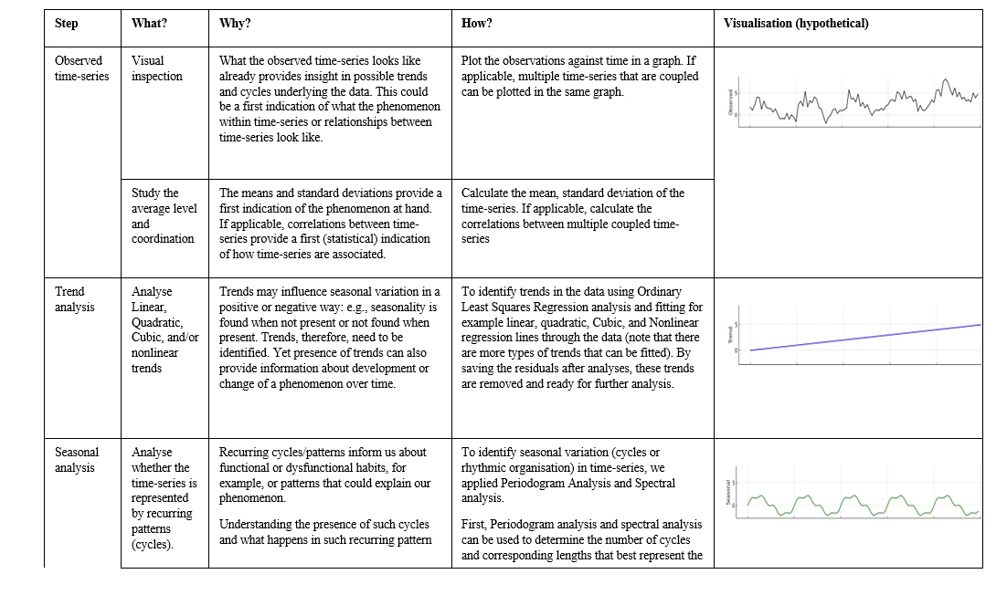
Warner (1998) identifies four steps in time-series decomposition when studying rhythmic organisation/seasonality in time-series (See Figure 1 for a schematic representation of the steps). The first step consists of two parts related to the inspection of the observed data: (a) the visual inspection of what the data looks like and (b) description of the data in terms of average level (i.e., means and standard deviation) and coordination (i.e., correlations between time-series). The second step is to study linear, quadratic, cubic, and nonlinear trends in the data using Ordinary Least Squares Regression analysis. The third step is to study seasonality to identify recurring patterns in time-series data and, if necessary, synchronisation between two coupled time-series using periodogram and spectral analysis. The fourth and final step is to study randomness of residuals, using the Cross Correlation Function and fitting Auto Regressive Integrated Moving Average (ARIMA 2,1,0) models.
Figure 1. Schematic representation of the four steps in time-series decomposition. The steps are presented in order of operation. The visualisations presented above each step are hypothetical time-series representing what each step in time-series decomposition is identifying: the observed time-series, a trend, cycles in the time-series, and random variation in the time-series.
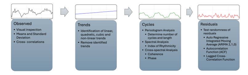
In this section, we will describe the various analysis steps (i.e., visual inspection and analysis of overall level and coordination, trend analysis, analysis of cycles, and random variation) needed to decompose the time-series data (see Figure 1 for a graphical overview of the steps). We will explain which information each step provides about the time-series that could help understanding the dynamics. In the next section, we will illustrate how the retrieved indices provide important information about teacher-student interaction and how teachers experienced it.
To get a first indication of the nature of the time-series and associations between time-series, one must first inspect the time-series visually, followed by calculating descriptive statistics to study the overall level within time-series and coordination between time-series.
2.1.1 Visual inspection of the time-series
When conducting time-series analysis, visual inspection of the time-series is a good and important starting point to get some qualitative sense about what is happening. For example, does the time-series appear to be affected by one or more trends, are certain peaks visible at certain time-points, and whether they seem to go together with peaks in other time-series, is there sufficient variability to explain, etc. Various types of visualisations can be used, such as sequence plots, in which the observations are plotted against time. It is possible to add multiple time-series in one sequence plot, so that visual associations between time-series can already be observed.
2.1.2 Overall level and coordination
To describe the overall level of time-series one can calculate the mean and standard deviations and the range (min/max) of the observations in the time-series. This provides a general idea about the observed phenomenon, both within-person and between-person.
A general statistic to describe overall coordination of time series is the cross-correlation statistic. When two or more time-series are observed, the correlation between these time-series can be calculated to study whether and how these are associated. Both the strength and the direction of the correlation provide information. Positive cross-correlations mean that the observations are moving in the same direction at the same time, and vice versa for negative correlations. The strength of the cross-correlation shows how strongly changes in the two time-series are connected. It should be noted though that cross-correlations have been critiqued for being highly affected by trends in the data. Regardless of this critique, the cross-correlations between the raw time-series already provide us with valuable preliminary information about associations between time-series. How to remove trends is described in the next step.
The next step in time-series decomposition is to statistically determine the presence of linear or curvilinear (e.g., quadratic - with one bend, cubic - with two bends) trends in the time-series. Trends can influence the exploration of cyclical patterns in the time-series data, such as wrongfully identifying cycles that are not really present in the data. Trends should therefore be identified and removed before proceeding with studying cycles in the data (Warner, 1998). Trend analysis can be done through curve fitting (e.g., Curve Estimation in SPSS).
In studies where the identification of cyclical trends is the sole purpose, these trends are often removed without examining them (Warner, 1998). For example, in studies on the business cycle what information trends can provide is of less interest, whereas predicting the length of cycles and when recessions will hit is more important. However, in the study of social interaction dynamics, trends can provide important information, for example about increasing or decreasing levels of positive emotions from moment-to-moment, or an increase of physiological arousal throughout a lesson.
Note that trends are not necessarily present in all time-series, or that the type of trends present may differ per time-series. Before proceeding to the analysis of cycles, all significant trends need to be removed from the time-series, since trends can affect associations between time-series and the identification of cycles. Of course, trends only need to be described or removed when present in the data. This means that for some time-series only a linear trend needs to be removed, whereas for others also quadratic, cubic, or even other types of trends need to be removed. Detrending the data is done through Curve Estimation and saving the residuals as new variables. The residuals can then be used as the dependent variable in the analysis of cycles.
To identify and analyse recurring patterns in time-series data is necessary to study the seasonality of time-series. For example, student motivation is often increased after a weekend or a period of vacation and declines when a new weekend or vacation approaches. Even within lessons motivation can vary. This is called seasonal variation and can be identified using spectral analysis (which is described in 2.3.1). Seasonal variation can also be associated with another variable. This can be analysed using cross-spectral analysis (which is described in 2.3.2)
2.3.1 Periodogram and spectral analysis
To identify the number and length of cyclical components that explain most variance in a time-series two methods can be used: periodogram analysis and spectral analysis (Warner, 1998). Both methods are based on the same principle of fitting sinusoidal wave forms (i.e., periods or cycles) to the data and obtain their explained variance. A time-series can be decomposed into N/2 sinusoidal wave forms with different period lengths (i.e., cyclical components, e.g., N/1, N/2, N/3 etcetera.). For this reason, the number of observations need to be an even number. For each of these cycle lengths, a Sum of Squares (SS) can be calculated as a periodogram intensity estimate;-. In essence the periodogram intensity estimate is a measure of explained variance per cycle length.
For example, for 200 observations of 5-sec intervals, this means that 100 SS terms are calculated (i.e., 200/2). The first cyclical component is then 100 observations long and has a duration of 8.33 minutes per cycle (i.e., (((200/2)*5s)/60)), the second cyclical component is 66.67 observations long (200/3) with a duration of 5.56 minutes per cycle, the third cyclical component is 50 observations long (200/4) with a duration of 4.17 minutes per cycle, and so on until the maximum of N/(N/2) (i.e., 200/100=2 observations long). By dividing the SS by the SStotal, the proportion of explained variance for each cycle length can be calculated. The cycle length with the largest explained variance indicates the best fitting cycle length for the time-series.
Spectral analysis differs from periodogram analysis in that with Spectral analysis the periodogram intensity is smoothed to account for possible sampling error, which is a pitfall of periodogram analysis. This means that a smoothing procedure is applied to replace each periodogram intensity estimate with a weighted average of a few neighbouring frequencies (Warner, 1998). A frequency is the proportion of cycles per observation (unit of time) and is calculated by 1/N (1/416=0.00240); Note that the frequency value is the inverse of the cycle length. Smoothing entails deciding upon (1) the width of the window of neighbouring frequencies (i.e., how long the cycle of interest is) and (2) the way weights are assigned to the frequencies in the window (Warner, 1998), which can be done using different methods (i.e., Hamming, Daniell, Bartlett, Tukey, and Parzen in SPSS). Deciding upon the smoothing procedure and the width of the window is a matter of choice (Warner, 1998). The larger the window, the more smoothed the time-series will become. See Table 1 for a worked example of what periodogram and spectral results look like for one of the cases.
Often in time-series, it can be seen that the explained variance in cyclical components next to the component with the highest explained variance (hence, the best fitting cycle length) is also relatively high. Which cyclical components are of interest is up to you (Warner, 1998). It does make sense to look into rhythmic variation across a larger number of cyclical components, for example by selecting a set of components that explain a significant amount of variance. Significance of explained variances per frequency is done with the Fisher test (Warner, 1998). Based on these explained variance an Index of Rhythmicity (IR) can be calculated (Sadler et al., 2009; Warner, 1998). The IR is derived by calculating the sum of the explained variances (g values, c.f. the variable gCT in Table 5) of all cyclical components selected in the set. The IR indicates how well an individual time-series is represented by cycles in the low-frequency end of the power spectrum; hence it represents the total proportion of variance explained by multiple but “a relatively small number of cyclical components” (Sadler et al., 2009, p. 1012) adjacent to each other. According to Sadler et al. (2009) an IR > .80 indicates that the cyclical variation represents the time-series well.
Table 1. Worked example of periodogram/power spectrum results for Communion of Teacher A.
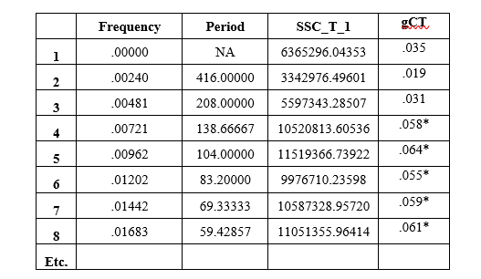
Note. SSC_T_1 = Sum of Squares per period for Teacher Communion. gCT = Explained variance SS/SStotal, where SStotal= 180297867.25. *Significant Fisher test value gCT for 416 observations and an = .05 is .03971 (Warner, 1998).
2.3.2 Cross-spectral analysis
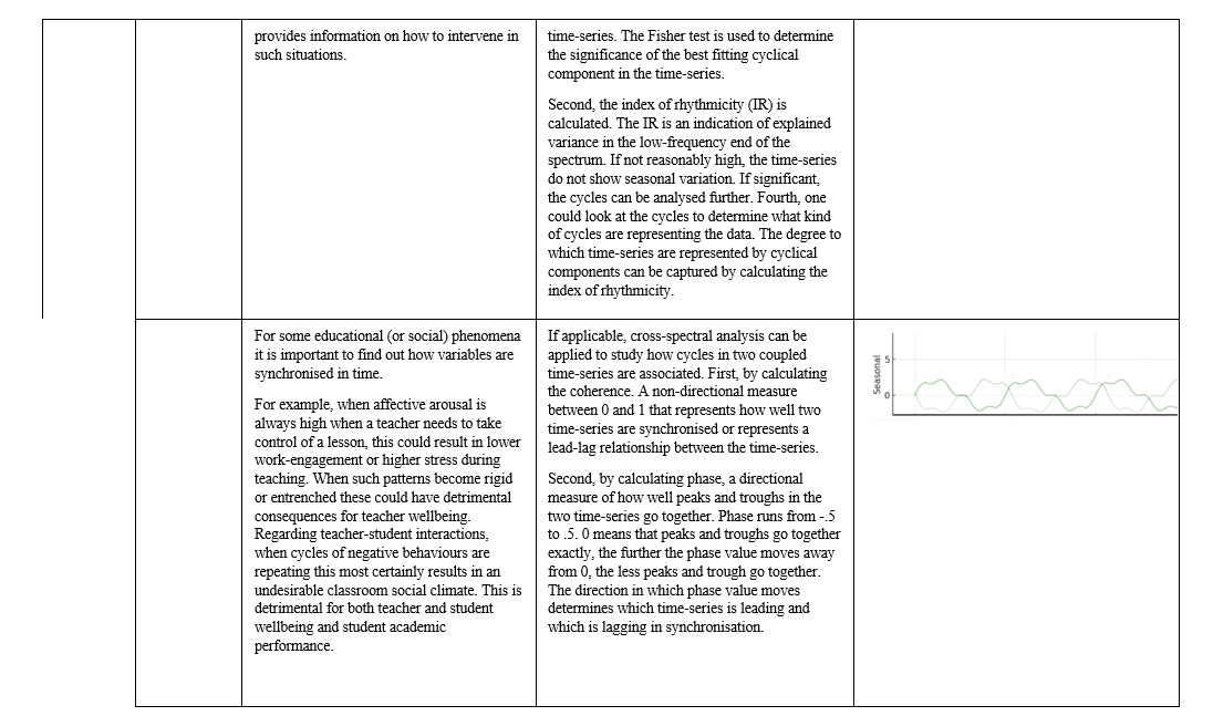
After identifying the cyclical components in the individual time-series data, it is possible to analyse two time-series together with cross-spectral analysis. In essence, cross-spectral analysis yields a cross-product of two smoothed power spectra, so the cross-product of the frequency values corresponding to two separate time-series (Warner, 1998). Thus, per cycle length the frequency of variable 1 is multiplied by the frequency of variable 2. To interpret the results of cross-spectral analysis it is necessary to calculate the indices of Coherence and Phase. Both values are based on these cross-product values and are calculated per cyclical component with the most optimal cycle length. In SPSS, cross-spectral analysis provides the coherence and phase values as new variables in the dataset.
Coherence is the correlation between two-time series at each individual cyclical component. The Coherence is non-directional and the value ranges from 0 = no synchronisation to 1 = maximum synchronisation. The squared Coherence is similar to an R2 serving as an estimate of percentage of variance that is predictable from one time-series to the other. This represents the degree of entrainment (i.e., synchronisation) between two time-series. That is, how well cycles in the first time-series go together with cycles in the second time-series.
Phase is an indicator for a lead-lag relationship. Per frequency the phase value indicates whether the changes in one time-series go together with the other, or not. Phase is reported in radians in the SPSS dataset and should be converted to fractions of a cycle. This can be calculated by dividing the Phase value by 2π. This results in values that lie between -.50 to .50, where a value of 0 means that the cycles peak at the same time, a value of -.50 or .50 means that peaks in cycles are opposite. The direction indicates which time-series is leading or lagging. A value of .50 means that the first time-series is leading half a cycle before the second time-series, -.50 means that the second time-series is leading half a cycle before the first time-series. When the cyclical component of the first time-series is 6.91 minutes long and the phase is .50, this means that first time-series is leading the second time-series by 3 minutes and 27 seconds. It should be noted that interpreting the phase value only makes sense if coherence is reasonably high. Thus, when coherence is negligible, interpreting phase is not informative, because cycles in one time-series do not explain variance in the other time-series.
Like with the IR in individual time-series, it is possible to average the coherence values for a larger set of cyclical components. According to Warner (1998), the best way to do this is by weighting the coherence values by the g values from the univariate analysis and calculate the average weighted coherence across the set of cyclical components of interest. Average Weighted Coherence is then the proportion of shared variance between time-series in the lower frequency band and represents how well the coupled time-series go together. Average Phase is a measure that represents the degree to which peaks in one time-series go together for a specific set of frequencies corresponding to the lower frequency band. The phase values in fractions of a cycle are averaged across the frequencies of interest.
Note that when calculating these averages, the number of most optimal cyclical components for the two time-series may be different. For example, for time-series X, a set of 16 cyclical components can be selected and for time-series Y, a set of 20 cyclical components might best represent the data. You can decide the best way to choose the set that best represents both time-series, for example by taking the average of 18 or by selecting the number with the smallest or the largest number of cyclical components (Sadler et al., 2009).
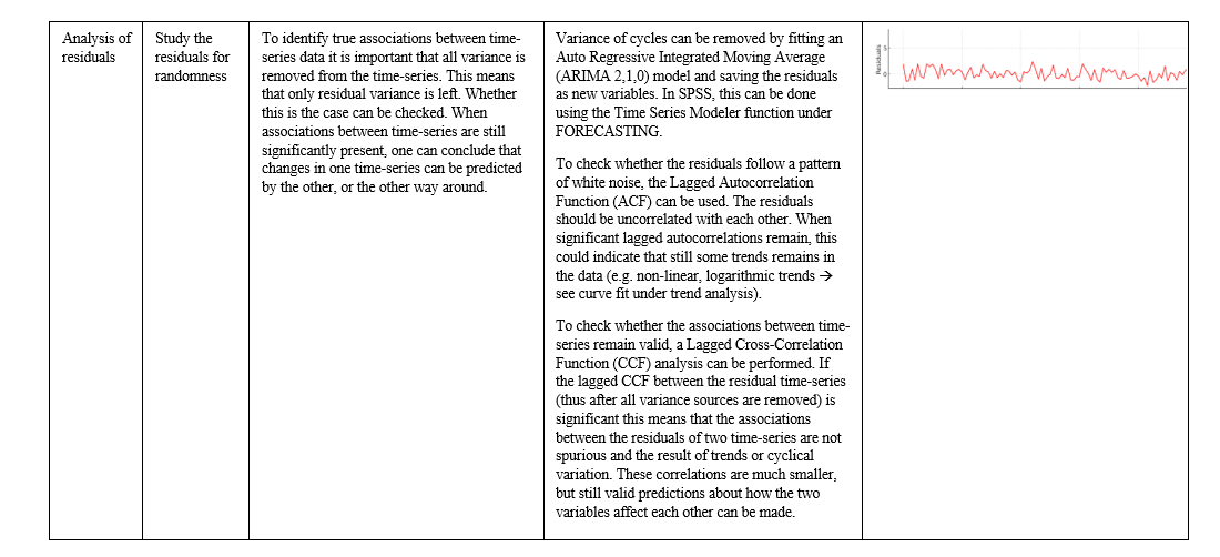
The final step in the process of decomposing time-series is to study the degree of random variation (or white noise) left in the residuals of the individual time-series after all trends and the cyclical variation are removed. This final step is used to determine whether all information in a time-series was analysed and interpreted, and no more variance is left to explain. This final step entails fitting an Auto Regressive Integrated Moving Average (ARIMA 2,1,0) model (Sadler et al., 2009; Warner, 1998). This can be easily done in SPSS using the Time Series Modeler function under FORECASTING. When saving the residuals, first the serial independence of the residuals can be checked by running a Lagged Autocorrelation Function (ACF). This analysis can be followed by a lagged cross-correlation (CCF) analysis to study the remaining association between residuals of two time-series. If the lagged CCF between time-series is significant, this means that the two time-series are still related after controlling for serial dependence. The remaining correlations most likely are much smaller, but valid predictions about the association between these variables can still be made. For example, hypothetically, in the first cross-correlation analysis between the raw time-series X and raw time-series Y, we saw a significant positive correlation. After removing all the variance components (i.e., trends, cycles) the correlation is not significant anymore. This means that the variance components affected the correlation significantly, where in reality there is no association between the two variables. Yet, if the correlation between X and Y remains significant, we can conclude that the association is true.
To illustrate the steps of time-series decomposition described in section 2, we will apply these steps in a worked example to data of four teachers with contrasting characteristics. The purpose of this methodological illustration is not to draw important empirical conclusions, but to guide researchers through the steps of time-series decomposition via a worked example. Therefore, in some places we have chosen to only provide examples for one or two teachers (e.g., visualisations) and in others we have included data for all four (e.g., results of the spectral analysis).
The classroom is a highly social and emotional setting. Good relationships between teachers and students foster a safe learning environment, are associated with higher teacher well-being (Spilt et al., 2011), higher student achievement and better socio-emotional functioning (Becker et al., 2014; Mainhard et al., 2018). Teacher-student relationships are however not static and linear (Mainhard et al., 2011), but dynamic and nonlinear, and develop through moment-to-moment interactions (i.e., interactions are the building blocks of relationships; Granic & Hollenstein, 2003). Yet, little is known about the moment-to-moment dynamics in teacher-student interactions, and how they affect macro-level outcomes. Assessing the temporal dynamics in interactions is important to grasp what happens in the classroom, when aiming to provide (individual) feedback to teachers, and to establish guidelines for beginning teachers.
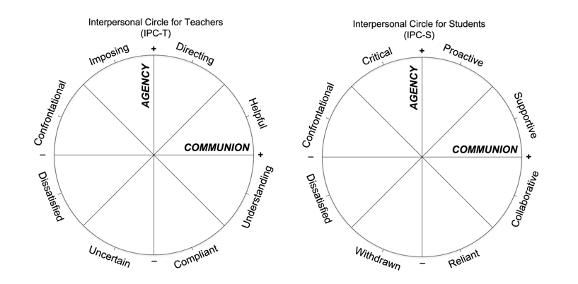
Teacher-student interactions and relationships are often studied using Interpersonal Theory (Kiesler, 1996). Interpersonal behaviour can be described using a two-dimensional model: the Interpersonal Circle (IPC). The first dimension is Agency and represents the degree of dominance vs. submission. The second dimension is Communion which represents the degree of friendliness vs. hostility. In Figure 2, two IPCs that describe respectively teacher behaviour (IPC-T) and student behaviour (IPC-S) are presented. Previous studies have shown that good teacher-student relationships are characterised by relatively high levels of teacher Agency and Communion, that is, being a ‘warm demander’ (Irvine & Fraser, 1998; Wubbels et al., 2006). Most previous research focused on trait-level teacher behaviour as an indicator for relationship quality, by using questionnaires to assess students’ perception of their teachers’ interpersonal behaviour (e.g., Wubbels et al., 2006). Such questionnaires cannot measure the more subtle changes in behaviour, which are essential to assess interaction dynamics in classrooms. Student perceptions also differ from how teachers view themselves or external observers would rate teacher behaviour (Donker et al., 2021). Therefore, in the present study, we observed moment-to-moment interpersonal behaviour of teachers and students, using a continuous coding method called Continuous Assessment of Interpersonal Dynamics (CAID; see Method section), which is rooted within Interpersonal Theory (e.g., Sadler et al., 2009).
Figure 2. Interpersonal circles to describe teacher (left) and student (right) behaviour (Pennings et al., 2018).
Such continuous coded time-series data allow for studying interaction patterns of teachers and students. Interpersonal theory states that good interactions generally follow the principle of complementarity (Kiesler, 1996). This means that how a person reacts to another person is not random, but contingent upon the behaviour of the interaction partner. All interpersonal behaviour includes an interpersonal bid that invites others to react in a certain manner. This interpersonal bid works differently for Agency than for Communion. In Agency, the interpersonal bid invites oppositeness in behaviour. This means that dominant behaviour tends to elicit submissive behaviour. In Communion, the interpersonal bid invites sameness. Friendly behaviour tends to elicit friendly behaviour (or hostile behaviour elicits hostile behaviour). It should be noted though, that complementarity in hostile behaviour is generally not beneficial for the quality of interactions and development of sustainable working relationships. Pennings et al. (2018) found indeed that teachers with good quality teacher-student relationships can refrain from complementarity in hostile situations, as compared to teachers with less preferred relationships. Time-series analysis can provide important information about complementarity in teacher-student interactions. We will discuss the information that each step in the time-series decomposition provides in light of identifying complementarity in teacher-student interactions.
Moreover, interaction does not only occur on the behavioural/observable level. How people behave is also related to how they feel, and vice versa, how they feel is affected by their behaviour. For example, teachers who feel very confident when providing students with more autonomy or anxious when having to take control may behave differently from those teachers who do feel enjoyment or anger in such situations. Collecting continuous self-reported data on emotional experiences is difficult, but also taps only into the conscious emotional experiences, thereby overlooking unconscious processes, such as appraisal processes (Scherer, 2009). Moreover, repeatedly reporting on emotions can be demanding and even affect feelings (Scollon et al., 2009). In this article we therefore include heart rate as a relatively unobtrusive measure of teachers’ affective arousal (Donker et al., 2023). Physiological measures such as heart rate of electrodermal activity can be used to measure affective arousal continuously (Kreibig, 2010; Van Dijk et al., 2013). Evidently, physiological measures are first and foremost indicators of biological changes related to physical activity and there is no one-to-one link between physiology and emotions (Kreibig, 2010). However, by controlling the heart rate signal for physical activity, the remaining physiological activation is likely associated with unconscious emotional processes or affective arousal (Myrtek, 2004). Therefore, we included physiological measures of teachers’ real-life emotional experiences to study how teacher’s behaviour is associated with their affect, as well as how teacher’s affective experiences are associated with student behaviours. To our knowledge, this is a first attempt to study the association between observations of teacher or student behaviour with teacher affective arousal using a CDS approach and spectral analysis of time-series.
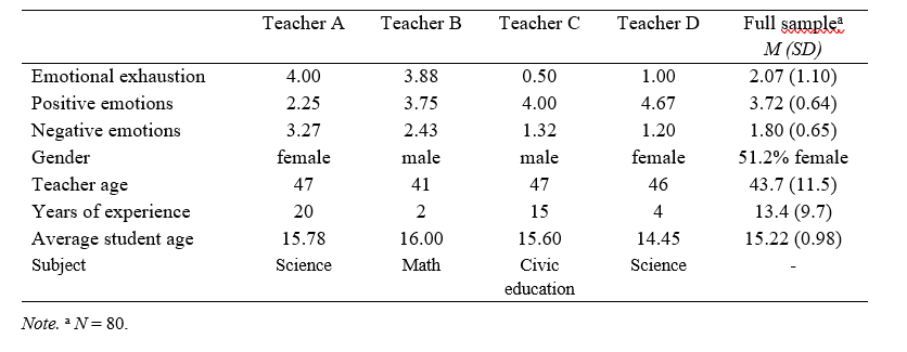
We selected four secondary-school teachers from a larger research project (Donker, 2020). We selected teachers who differed in their self-reported emotional exhaustion and emotions to maximise the potential variation in teacher-student interaction processes during their lesson. We included two female and two male teachers between the ages of 40 and 50, but with different years of teaching experience, again to maximise variation (see Table 2).
Table 2. Descriptive statistics.
In the larger study, teachers were recruited individually via different channels. Participating teachers were observed during one regular classroom lesson which lasted about 50 minutes. Simultaneously, teachers’ physiological activation was measured. All lessons included some plenary instruction by the teacher after which the students worked individually or in small groups on an assignment. At the end of the lesson, both teachers and students completed a questionnaire. Teachers received a personalised report of their questionnaire data and a gift card after their participation.
Teacher and student interpersonal behaviour. Teacher and student interpersonal behaviour was coded from a video recording of the lesson. Different cameras were used for observing teacher behaviour (in the back of the classroom, linked to a microphone that the teacher was wearing) and for student behaviour (in the front of the classroom), so that we could also observe non-verbal/facial expressions of the students. Students who did not provide consent for being recorded were in a corner of the classroom that was not captured on video. To observe moment-to-moment behaviour of both the teacher and the students, we used Continuous Assessment of Interpersonal Dynamics (CAID), also known as the joystick method (Lizdek et al., 2012; Sadler et al., 2009).
Figure 3. Continuous assessment of interpersonal behaviour (Pennings et al., 2014).
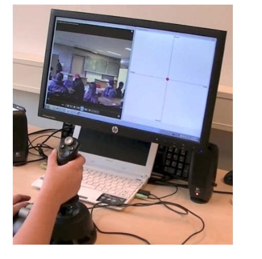
With CAID, a computer joystick apparatus and corresponding software (i.e., Joymon) are used to continuously code the level of Agency and Communion in interpersonal behaviour while watching the video recording. Joymon generates a Cartesian plane representing the IPC (see Figure 3). By moving the joystick in the desired direction , behaviour coordinates (i.e., Communion on the x-axis and Agency on the Y-axis) are automatically recorded in a log file. This means that the observers can keep watching and observing the behaviours without interruptions of pausing/unpausing the video.
The automatic recording of the behaviour coordinates occurs every half second, by default, resulting in time-series of observed behaviours. The behaviour coordinates range from -1000 = very low Agency/Communion to +1000 = very high Agency/Communion, to ensure maximum sensitivity of the joystick while coding. The position of the joystick in the Cartesian plane represents the type of interpersonal behaviour that is being coded. The distance of the joystick cursor’s location from the origin indicates the intensity of this behaviour. For example, when someone dominates the conversation, this would be coded as high in Agency, whereas following what others are demanding would be coded as low in Agency. Smiling or supporting would result in an increase in Communion and ignoring students or making ‘cold’ comments results in a decrease of Communion (Ross et al., 2017). Note that Agency and Communion are coded at the same time because all interpersonal behaviour should be described by both dimensions simultaneously. For example, someone can be dominant but friendly at the same time (e.g., being leading or supporting) or be submissive and hostile at the same time (e.g., being passive aggressive).
Each video was coded by three trained observers. Teacher and student behaviour were coded separately by a different team of coders. The second author and two other observers were initially trained by the first author who was trained by Pamela Sadler and who is an expert in CAID for observing teacher-student interactions. The initial training session consisted of familiarizing the observers with the interpersonal circle and the joystick and how it moves. For example, by moving the joystick to the correct location of a list of interpersonal behaviours (e.g., leading, warm, introverted, critical) and observing short videos ranging from 1 to 5 minutes in duration, that are always being used for this training. Ratings of the coders were compared to ratings of other coders trained with these videos. Coders were also informed about pitfalls and biases that can occur during coding. After initial training, observers engaged in three subsequent in-person sessions in which coders got more familiar with the interpersonal circle and coded longer example video fragments. Differences between coders were extensively discussed. Also, during the coding process, there were calibration sessions in which the coding was discussed to prevent coder drift. Coders could only start formal coding when they scored reliable on a training set of videos. This is especially important, as coders could not pause their coding, but coded continuously until the video was finished.
Most videos could be coded by watching the video just once. We calculated reliability by calculating the Intraclass Correlation Coefficient (ICC(k)) between the continuous ratings of the three coders (ICC(k=3); LeBreton & Senter, 2008). ICC is a value between 0 and 1, and is deemed insufficient when below .50, moderate between .50 and .75, and good or excellent when above .75 and .90, respectively (Koo & Li, 2016). When the reliability of their coding was insufficient (ICC <.60; note that this is more rigorous than suggested by Koo & Li, 2016), the most deviating coders redid the coding or a fourth independent coder was included. The time-series of the three most reliable codes were averaged for the analyses to dampen idiosyncratic observations of individual observers. For each of the videos an ICC value was calculated, but here we report the average ICC for all coding of the selected teachers. ICC(k=3) was .61 (SD=.07) for Student Communion, .66 (SD=.08) for Teacher Communion, .71 (SD=.21) for Teacher Agency, and .79 (SD=.13) for Student Agency, which is sufficient and comparable to other studies (Pennings et al., 2018; Sadler et al., 2009).
Teacher affective arousal.Teachers’ affective arousal and their physical activity during teaching were measured using the VU University – Ambulatory Monitoring System (VU-AMS; vu-ams.nl). Before the lesson started, seven electrodes were attached to the teacher’s chest and back to measure the Electrocardiogram (ECG). After signal inspection on a computer, teachers could wear the device in a belt and move freely around the classroom. After the lesson, the ECG data was imported into the VU-DAMS software program and automatically checked for irregularities and outliers. Artefacts were manually corrected if necessary (less than 1% of the data).
The raw heart rate signal was controlled for the physical activity of the teacher using an Additional Heart Rate approach (see Donker et al., 2018 for details). The resulting heart rate data is a measure of the teachers’ heart rate beyond the level that could be expected based on their physical activity. This measure can thus be seen as a measure of affective arousal (Myrtek, 2004).
We exported the heart rate data per 5 sec. Five-second time periods seem most adequate, as they form a nice balance between getting precise information on dynamic changes and providing reliable data, as five-second periods include several heartbeats (see also Donker et al., 2018). Note that using 0.5 sec intervals (in line with the CAID data) for the affective arousal data is not possible, because most people have only one heartbeat every second (with a mean heart rate of 60 bpm). Also, using 1-sec intervals would have resulted in missing data for some participants (who have even lower heartbeats). Moreover, 1-sec intervals would have resulted in more random variation. Using 5-sec intervals has been proven to be a valid interval for reliable, but sensitive HR data (see Donker et al., 2018). The CAID data was aggregated to the 5-sec level as well to match the physiological data for analysis.
The time-series analysis was conducted in SPSS (version 27). We only analysed datapoints with complete data for all three sources (teacher affective arousal, teacher interpersonal behaviour, and student interpersonal behaviour). This is necessary for the spectral analysis, which cannot handle missing data or time-series of varying lengths. This means, that for some data we had to truncate the time-series to match the length of the shortest time-series in the set. For example, if the video of the teacher covered 38 minutes of the lesson, the student video 39 minutes because it was stopped one minute later, and the affective arousal measurement was 40 minutes, then the student behaviour and affective arousal time-series would be shortened to 38 minutes to match the teacher behaviour time-series.
We will discuss which information each step in the time-series decomposition provided about the four teachers in this example.
4.1.1 Visual inspection of the time-series
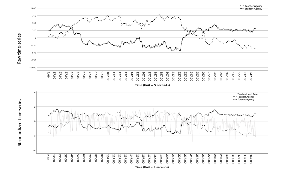
In Figure 4 and 5, the visualisations of the time-series for Teachers B and C are provided as an example. Figure 4 shows that in general peaks in teacher Agency went together with troughs in student Agency, and the other way around (i.e., complementarity). In the beginning of the interaction, Teacher B was somewhat neutral in Agency, while the students were dominant. After a few minutes the teacher became more dominant, and the students became more submissive. This is often an indication of the teacher starting the lesson and starting to provide instruction. This pattern lasts for a large part of the interaction, after which the students become more dominant, and the teacher becomes more submissive. In general, this indicates that Teacher B provides students room to ask questions or puts them to work independently.
For Teacher C (see Figure 6), the time-series for communion show some indication of sameness, but peaks and troughs do not necessarily seem to go together. However, the teacher and students are friendly during the entire interaction. Probably decreases in friendliness of the teacher did not affect communion of students because his behaviour was still relatively friendly.
Figure 4. Time-series corresponding to the levels of Agency for teacher B and his students. The upper panel presents the raw time-series of teacher and student behaviour. The lower panel presents standardised time-series so that the teacher heart rate time-series is visually comparable to time-series of interpersonal behaviour.
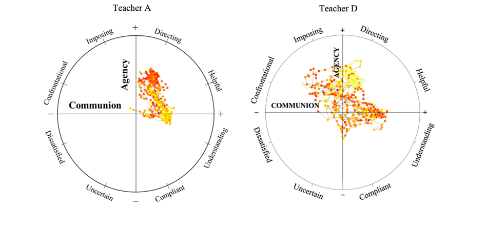
For Teachers A and D, we plotted the time-series of teacher agency and communion during the lesson on the Interpersonal Circle as another illustration of the data (see Figure 6). Teacher A mainly showed positive levels of Communion during the lesson (i.e., all the dots are on the right side of the circle). Teacher D showed a more varied pattern of interpersonal behaviour, including lower communion at several times. Additionally, teacher heart rate at this particular moment (i.e., the combination of Agency and Communion) is represented by the colour shading of the dots (i.e., darker colours/red indicate a relatively higher heart rate and lighter dots/yellow indicate low heart rate). Figure 6a thus shows that Teacher A’s heart rate was high mainly when showing high levels of agency and somewhat lower (but still positive) levels of communion. For Teacher D, the pattern for the teacher agency-heart rate is exactly the other way around (see Figure 6b). This teacher showed an increased heart rate mainly at lower levels of agency, suggesting that different behaviour might be arousing/challenging for teacher A and D.
Figure 5. Time-series corresponding to the levels of communion for teacher C and his students. The upper panel presents the raw time-series of teacher and student behaviour. The lower panel presents are standardised time-series so that the teacher heart rate time-series is visually comparable to time-series of interpersonal behaviour.
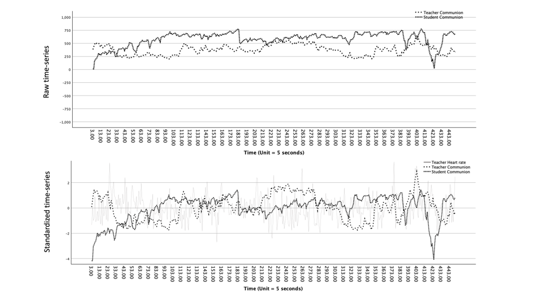
Figure 6. Associations between heart rate and teacher Agency and Communion of Teacher A and D.
4.1.2 Overall level and coordination
The overall level (i.e., means and standard deviations) of the behavioural and heart rate data are presented in Table 3. For Teachers A and B, students’ overall agency levels were relatively high, while student communion was low, compared to Teachers C and D. Teacher agency was overall the highest for Teacher C, while Teacher B scored highest on teacher communion. Teachers differed also in their average heart rate during the lesson, which might be related more to general fitness than social-emotional or classroom-related factors. Although these overall patterns give us some general insights in processes during the lesson, they do not grasp the dynamics of their behaviour during the lesson.
Both the strength and the direction of the overall coordination in time-series are indicative for the degree of complementarity in these cases. In Table 4 we present the cross-correlations between the raw time-series as well as the cross-correlations after removing the linear trend and after removing the linear, quadratic and cubic trends (detrended cross-correlations) to show the effect trends can have on the cross-correlations for our teachers. Thus, the correlations between the raw time-series might be inflated by trends in the data. We therefore suggest to mainly interpret the detrended correlations (in this case those under the ‘detrended all’ column in Table 4). Yet here we will first look at the raw time-series to get some first idea about the descriptive data. The interpretation of the detrended correlations will be discussed after the next step in which trends are removed from the data.
4.1.2.1 Interpretation of the correlations between the raw time-series
For all teachers, the cross-correlation between student agency and teacher agency was negative, indicating oppositeness, which is in line with the principle of complementarity. For Teacher A, the levels of oppositeness in agency were lower compared to the other teachers. For Teacher B, the level of oppositeness was very high, which corresponds to our visual inspection (see Figure 4). Teacher and student communion were positively linked for Teacher A, B, and D (i.e., complementarity). For Teacher C, the cross-correlation was not significant, indicating that teacher and student communion functioned rather independently, which we already saw in the visual inspection (see Figure 5).
Regarding the cross-correlations of Agency and Communion with heart rate, we found that for Teacher C, there were almost no associations between interpersonal behaviour and heart rate. On the other hand, for Teachers A, B, and D, the detrended cross-correlations with Agency were stronger, but still low, both for teacher and student Agency. Heart rate was hardly correlated to communion in both teacher and student behaviour. This suggests that teachers’ heart rate is mainly associated with the level of Agency.
The visual inspection in the first step already provided an indication of the presence of trends in time-series. For example, Figure 4 hints at a cubic or nonlinear trend in the data, and although visually very subtle, Figure 5 does hint towards the presence of at least a linear trend in the data. The Curve Estimation analysis for our cases showed that the quadratic and the cubic terms significantly increased the explained variance compared to the linear model, but the degree to which variance was explained differed substantially (Table 5). Only for Teacher C, the heart rate did not follow any trend and student Agency did not show a linear trend. Of course, trends only need to be described or removed when present in the data. This means that for some time-series only a linear trend needs to be removed, whereas for others also quadratic, cubic, or even other types of trends need to be removed.
Table 3.Overall level of teacher and student Agency and Communion and teacher heart rate.
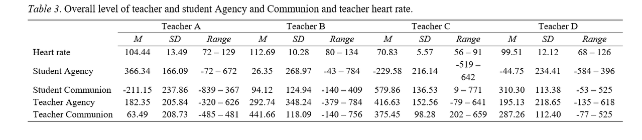
Table 4.Raw and detrended cross-correlations.
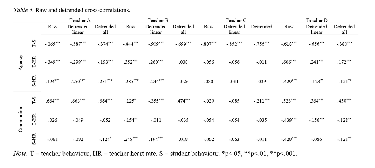
Table 5.Trend analysis results.
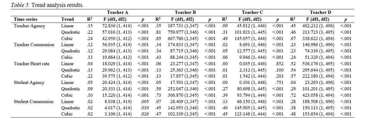
Figure 7.Graphs of the cubic trends in the time-series for each teacher and class. The y-axis corresponds to Agency (left panel) and to Communion (right panel); the x-axis corresponds to time (units = 5 seconds).
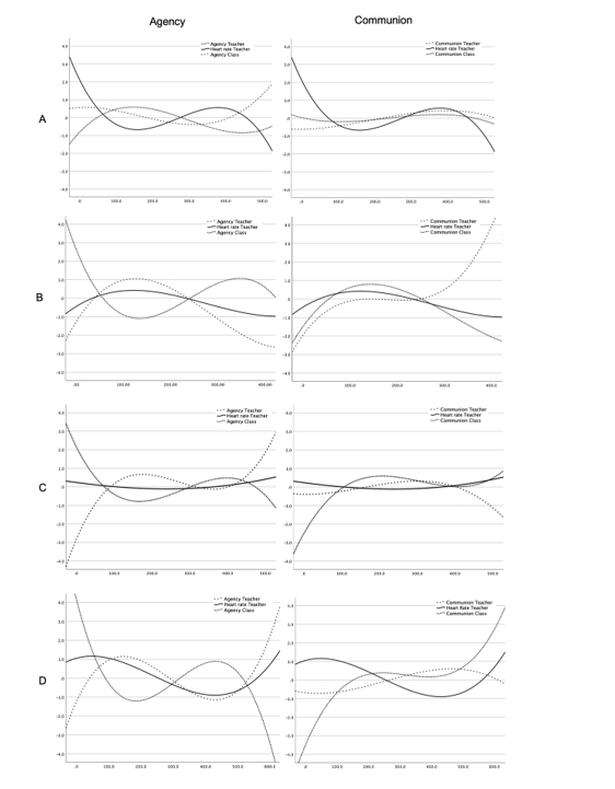
To examine the trends as Warner (1998) suggests we provided graphs of trends for all four teachers in Figure 7. We chose to provide the cubic trends, for the teacher, student, and heart rate in one graph instead of showing the linear, quadratic and cubic trends per time-series, because the combination of how the trends look between coupled time-series is more informative to us. Separate graphs are presented for Agency and Communion but note that teacher HR is added to all graphs (Figure 7).
When looking at the graphs of Agency for Teacher B, Teacher C, and Teacher D, the students start off being dominant (high Agency) and the teacher is submissive (low Agency). After about five to eight minutes, gradually the teacher becomes more agentic while the students become more submissive. This could mark the actual start of the lesson. After that moment, the trend-lines for these teachers and their class, clearly show an alternating pattern of dominance and submission in teacher and student behaviour. The fluctuations in the time-series seem to follow the complementarity principle of oppositeness. For Teacher A, the graph shows a somewhat different pattern, where the teacher starts of being more dominant, and the bends in the time-series are less prominent and alternating. The time-series seem to move together more, a pattern that for this and the other teachers can also be seen in the Communion time-series, which 4.indates sameness.
Before proceeding with the analysis of cycles, the trends need to be removed from the time-series, since trends can affect associations between time-series and the identification of cycles.
4.2.1 Interpretation of the correlations between the detrended time-series.
Table 4 shows how this works for the associations between time-series. For example, detrending affected the strength of the cross-correlations for several time-series of the different teachers, and this can go both ways. For Teacher A the correlation between teacher Agency and student Agency became somewhat stronger after removing trends; for Teacher B the correlation between teacher Agency and Heart Rate goes from a medium effect to a small effect after removing the linear trend, and to no effect after also removing the quadratic and cubic trends. Also, for Teacher B the cross-correlation between teacher Communion and student Communion changes from a small effect to a medium effect and even a stronger medium effect after removing the trends. In some cases, removal of trends did not affect the cross-correlations. These differences show the importance of detrending the data before drawing conclusions and proceeding with the analysis of cycles.
4.3.1 Spectral analysis
In our illustration we based the choices for smoothing procedure and window width on Sadler et al. (2009), who used similar data to ours. This means we used the Hamming procedure to assign weights, and a window of 5 neighbouring frequencies. The Hamming procedure attributes larger weights to the nearest frequencies and lower weights to the furthest frequencies within the window. In our analysis the two frequencies furthest away (T-2 and T+2) received a weight of 2.239, and those in between (i.e., T-1, T0, T+1) received a weight of 2.40. When performing this analysis in SPSS these weights are attributed automatically when choosing the Hamming procedure. To illustrate this, Table 1 shows the first 8 rows (low frequency-end of the power spectrum) of the smoothed results from the spectral analysis for Teacher Communion of Teacher A.
To determine the best fitting cycle length for the time-series in our illustrative example, we looked at the cycle (frequency) with the highest explained variance that was significant when we performed the Fisher-test (Warner, 1998). The results showed that the cyclical variation was significant in all Agency and Communion time-series. Teacher heart rate was not represented by significant cyclical variation for Teacher B and Teacher C. It therefore does not make sense to interpret cyclical patterns in the heart rate data for these two teachers (Warner, 1998).
Remember that it makes sense to look into rhythmic variation across a larger number of cyclical components by selecting a set of components that explain a sufficient amount of variance (i.e., using the Fisher test) and determine its degree of rhythmicity. In our study we chose to use the calculate Index of Rhythmicity (IR) based on the values corresponding to the cycle lengths that explain at least 1% of the variance in the time-series. The IR is derived by calculating the sum of g values (i.e., explained variances per frequency, gCT in Table 1) for a number of cyclical components (neighbouring frequencies) of interest. By selecting a set of cyclical component that explain sufficient variance in the time-series the IR represents the degree to which the identified set of cyclical components significantly represent the data.
Remember that it makes sense to look into rhythmic variation across a larger number of cyclical components by selecting a set of components that explain a sufficient amount of variance (i.e., using the Fisher test) and determine its degree of rhythmicity. In our study we chose to use the calculate Index of Rhythmicity (IR) based on the values corresponding to the cycle lengths that explain at least 1% of the variance in the time-series. The IR is derived by calculating the sum of g values (i.e., explained variances per frequency, gCT in Table 1) for a number of cyclical components (neighbouring frequencies) of interest. By selecting a set of cyclical component that explain sufficient variance in the time-series the IR represents the degree to which the identified set of cyclical components significantly represent the data.
For the four teachers the best representing cycle lengths varied from 3 to 6 cyclical components per lesson (ranging from the shortest cycle of 6.91 minutes to the longest cycle of 12.42 minutes). The IR values for teacher and student Agency and Communion are presented in Table 6. The IR values indicate that not all time-series are well represented by cyclical variation, especially in case of heart rate.
Table 6. Cross-spectral analysis.
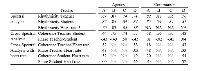
Note. * For heart rate only 4 values are available, these are presented in the Agency columns but not associated with Agency. NA = Not Applicable (because there is no cyclical variation in heart rate for these teachers). Rhythmicity and Coherence values lie between 0 and 1, where 1 indicates a high degree of cyclical variation for rhythmicity and a high level of entrainment for Coherence. Phase values lie between -.50 to .50, where a value of 0 means that the cycles peak at the same time, a value of -.50 or .50 means that peaks in cycles are opposite. The direction indicates which time-series is leading or lagging (Sadler et al., 2009).
4.3.2 Cross-spectral analysis
When using cross-spectral analysis it is useful for interpretation purposes to couple the cyclical components of the two time-series, by selecting the cyclical components that best fit both time-series. We synchronised the cyclical components of interest by using the average over the best cycle lengths as a cut-off point for two time-series.
Average weighted coherence. The cross-spectral analysis showed some variety in Coherence, thus coupled time-series were not all synchronised perfectly. For Agency, the entrainment between teacher and student behaviour is large for teacher B and C and medium for teacher A and D (Cohen, 1992). For Communion, the degree of entrainment is moderate for all teachers. Thus, for all teachers, the cycles in teacher behaviour go moderately together with cycles in student behaviour. Especially the time-series coupled with heart rate were low to moderately synchronised. Remember that for Teacher B and C heart rate was not cyclical, therefore we did not perform cross-spectral analysis on these data. Cycles in teacher heart rate and teacher behaviour and in teacher heart rate and student behaviour, for teacher A and D, were entrained moderately to large (values ranging from .18 to .56). Thus, teacher heart rate seems not overly related to or affected by cycles in their own behaviour or their students’ behaviour. Yet Teacher D’s heart rate was stronger related to increases or decreases in teacher and student behaviour than Teacher A’s heart rate was.
Average Phase. Average phase represents which variable is leading and which one is lagging in the interaction . Concerning teacher and student Agentic behaviour, teacher A, B and D were following the students and teacher C was leading the students. In all four cases by almost half a cycle, thus for all four teachers the peaks in teacher behaviour went together with troughs in student behaviour and the other way around. For Communion we saw a different pattern. For teacher A, B, and D, the phase values of almost 0 indicate that the peaks in teacher Communion went together with peaks in student communion, but there was no clear lead-lag relationship, although teachers A and D are leading slightly by a very small fraction of the cycle. For Teacher C, the students were leading and peaks in student communion went together with troughs in teacher communion, and the other way around. Note that this does not mean that the teacher was unfriendly. Both Table 2 and Figure 4 show that teacher C’s and his students’ behaviours were never hostile, but the raw time-series in Figure 4 shows that the degree of friendliness varied somewhat in an alternating manner.
For Teacher A the Coherence values with heart rate were quite small, therefore it does not make sense to interpret phase for this teacher. For Teacher D we can see that teacher Agentic behaviour is lagging very slightly with respect to the change in heart rate. We do see that changes in student agentic behaviour are leading changes in Teacher D’s heart rate. In case of Communion, we see that teacher and student behaviour both precede changes in teacher heart rate.
In the fourth and final step we checked whether all variance and serial independence was removed from the data with these steps of time-series decomposition. To do this we fitted an ARIMA model to each individual time-series. The results of our ARIMA analysis showed that almost all time-series consisted of white noise, and that only a very small amount of variance was left in the time-series (Table 7). This means, that still some variance remained in those time-series that should be looked into further. Since the purpose of this paper was to illustrate the steps of time-series decomposition, we only looked at linear, cubic, and quadratic trends in the current time-series in the trend analysis step, but other trends such as nonlinear or logarithmic trends may also be present. These could be further investigated.
To assess whether conclusions about associations between the remaining time-series can be made we calculated cross-correlations using the Cross Correlation Function in SPSS. Several cross-correlations between the residuals of the time-series were not significant, indicating that for those variables no further associations between the time-series were present. This means that the associations found in step 1 were inflated by trends and cyclical variation, rather than true association. Yet several associations between the residuals of various time-series remained significant , after all sources of variance (i.e., trends and cycles) were removed, which means that for those time-series we can make true inferences about their associations. Hence, the association is not a result of variances in the data that spuriously affect the association. For teacher A and B both teacher Agency and Communion were still associated with student Agency and Communion, which corresponds to the theoretical assumption of complementarity. But note that for Teacher B some variance still remained in the time-series for Teacher Communion and for Teacher A in Student Agency (Table 7), therefore conclusions should be drawn carefully. Yet, for teacher C only teacher and student Agency was significantly associated. This means that the theoretical principle of complementarity does not always hold; it did for teachers A and B, but only partly for teacher C. Also, for teacher D only teacher and student Communion were significantly associated but note that here the ARIMA analysis showed significant residual variance. These time-series should be studied further before valid predictions can be made. For teacher B, C and D, teacher heart rate remained associated to teacher and/or student behaviour, but for these teachers residual variance was found fitting the ARIMA model. The remaining correlations could indicate that for these teachers interpersonal behaviour of teachers themselves or the students was related to decreasing or elevating heart rate, as a proxy for affective arousal but this should be studied further. Also, note that for Teacher B and C the heart rate time-series did not follow a cyclical pattern. That does not mean that they should not be considered anymore after all variance is removed from the time-series. Still associations with other time-series may be present, but the variance does not come from cyclical patterns (Warner, 1998).
Table 7. Results of the ARIMA analysis.
The findings described above deepen our understanding about the individual differences in real-time teacher-student interactions. Our results showed that all four teachers are very different in terms of how social interactions occurred and how heart rate was related to their own and their students’ behaviour. Instead of looking for generalised causes or solutions, we as social and educational scientists should embrace these differences. Being able to study and understanding how individuals react to changes in the environment might be essential to help individual teachers improve their practice or prevent/overcome emotional exhaustion. Taking into account that we have only looked at one lesson of these teachers, different lessons will most certainly yield different results. This illustrates the importance of idiographic research over nomothetic research in trying to understand the temporal dynamics in educational phenomena.
The teachers who were selected for this illustration differed in certain characteristics like emotional exhaustion and teaching experience. Differences in their interactions or how heart rate is related to their behaviour could be related to these characteristics. For example, when for a teacher heart rate always increases when having to be agentic during a lesson, this could have an effect on exhaustion (or the other way around). For teacher A with a high level of emotional exhaustion, heart rate was not related to behaviour, but for teacher B it was. For teacher D who scored low on emotional exhaustion, heart rate was also positively related to teacher agency. It would be interesting to find out in more detail how signs of affective arousal affect these teachers’ emotional exhaustion.
Although heart rate is always cyclical, we did not find rhythmic variation in the low-frequency end of the spectrum for heart rate for teachers B and C. Given that heart rate in nature is cyclical, this could mean that the changes in heart rate for these teachers were not cyclical but only affected by incidents during the lesson. It could be valuable to study the effect of certain things that happen in lessons of these teachers.
For these two teachers the Phase value was also interesting. For Agency, Teacher B (higher on emotional exhaustion) was leading the students in Agency and Teacher C (lower on emotional exhaustion) was following the students, both for almost half a cycle. This could mean that teacher B is working too hard to guide the students, or that the students in teacher C’s class are easier to work with. These are interesting questions to study further, for example, by looking qualitatively what happens during the lessons, or through follow-up interviews with teachers using stimulated recall.
According to interpersonal theory, behaviours are always a combination of both Agency and Communion. Therefore, it is a limitation that we could not couple the time-series of teacher Agency and Communion into one time-series. Given that these observations are coordinates in a Cartesian plane, it is possible to convert the observations into one combined point per observation (see for example, Pennings & Hollenstein, 2020). However, this results in loss of information about the intensity of behaviours that cannot be captured in that same time-series. In the future, new ways of combining Agency and Communion into one time-series without losing information should be developed, for example, using cylindrical data analysis (Cremers et al., 2020). For now, we are confident that analysing the time-series separately and using cross-spectral analysis provides us already with valuable information about dynamics and fluctuations in the interactions.
Historically, educational and social scientific research was mainly nomothetic, looking at means and group level outcomes. Such analyses could lead to wrong interpretations and conclusions (Hilpert & Marchand, 2018), when researchers focusing on studying between-person outcomes try to generalise their findings to within-person outcomes. Yet social phenomena can hardly ever be generalised across the entire society. That is, individual differences are inherent to environmental, contextual, and cultural influences on social and educational phenomena (Hamaker, 2012; Murayama et al., 2017). This calls for a more idiographic approach (Hilpert & Marchand, 2018).
Fortunately, the focus of educational and social scientist is currently moving towards studying dynamics, fluctuation, and processes within systems instead of learning outcomes only. In educational and social sciences, many phenomena are complex and can be represented as time-series. Yet analysis methods stemming from complex dynamic systems theories, such as time-series analysis, are hardly ever used in these fields. One reason might be that researchers are unfamiliar with time-series analysis and discouraged by their seemingly complicated application. Another reason might be that the type of data that needs to be collected. Time-series data can be overwhelming and time-consuming to collect, depending on the phenomenon of interest and the method of data collection. To tackle the first problem and help social and educational scientists, we illustrated how the various steps of time-series decomposition are performed and can provide information about social interactions between teachers and students and teachers’ affective arousal (i.e., heart rate) in classrooms. We will discuss the possibilities of time-series decomposition here as well as some guidelines for starting with time-series research and analysis. With that we aim to lower the threshold to start such analyses. Furthermore, we aim to inspire social and educational scientists to engage more in idiographic research by discussing other educational phenomena that can be analysed using time-series analysis. We will also provide suggestions for other analysis techniques rooted in complexity theory.
To guide researchers in how the steps in time-series decomposition can inform their research we have schematically described the steps to illustrate the broader applicability of time-series decomposition beyond our own data in Table 8. We have also added a SPSS syntax in which all essential steps are added in a supplemental file (Supplemental file 1).
When engaging in idiographic research instead of nomothetic research there are no requirements in terms of sample size in participants, but it is important to investigate the sample size of data points. When starting out with collecting time-series data note that - as a rule of thumb – often 50 datapoints is mentioned. To use spectral analysis, there is no set rule and some other analysis techniques do not require this many observations (see the previous section). For spectral analysis, to determine the required number of data points one should think about the longest expected cycle underlying the phenomenon under investigation. According to Warner (1998) at least five but preferably over 10 cycles should be present in the data. So, for daily measurements with an expected cycle of 7 days in duration, at least 35 but preferably 70 (or more) daily measurements should be collected.
The choice of sampling frequency (time) is also open. It depends on what makes most sense to answer your research question (Singer & Willet, 2003). Given that interactions can change in a split second, it made sense for us to collect data every half-second, but measuring heart rate every half-second did not make sense, because most people have one heartbeat per second, and even measurements every second would yield missing data. When studying other phenomena different sampling frequencies may fit, for example when measuring sleep quality, one measurement per day will suffice or when studying academic performance, weekly or monthly measurements could suffice (depending on the research questions).
In this article we have illustrated time-series analysis using data on teacher-student interactions and teacher affective arousal. However, time-series analysis can be used in a broad range of educational phenomena, but in many cases calls for a shift in thinking about data collection when they require (intensive) longitudinal data collections. Some data are inherently longitudinal, such as learning analytics data or eye-tracking data, e.g., when studying learning processes and daily performance measurements of learning activities or weekly measures of performance are recorded as learning analytics data. When teachers’ use of learning analytics data in dashboards is studied, one could also record sequences of clicks on information sources or eye-tracking data to study what teachers are looking at. Such data sources are very suitable for studying using a CDS lens and various types of time-series analysis. Motivational processes or self-regulated learning could also be studied. For example, Garner and Russel (2016) studied self-regulated learning strategies through identifying patterns in learning behaviours of students during a self-paced learning task. Also, in general self-regulated learning is seen as a cyclical process consisting of three phases (forethought/planning phase, performance phase, and reflection phase; Zimmerman, 2002). Observations of self-regulated learning behaviours over time could provide valuable insight into the cyclical dynamics of self-regulated learning, that is, is self-regulated learning indeed merely cyclical, or does it consist of back-and-forth activities between phases. Currently, trace data or gaze data in digital learning environments are often collected over time to study this (Raković et al., 2024). Other data are not inherently longitudinal but very suitable for applying moment-to-moment data collections. Videos, which were used in the present study, or audio recordings are very suitable for example. Observing and analysing these as time-series requires a shift in thinking though. In the present study we have used a device that recorded every half-second the location of our cursor in the interpersonal circle. Van Heese et al. (2025) have used the same device to observe primary school teachers’ autonomy supportive behaviour. But other types of continuous observations are also possible. For example, Van der Steen (2014) coded every utterance in one-on-one researcher-child conversations about scientific concepts. Hendrickx et al. (2025) recorded changes in conversational moves during teacher-teacher collaborative group work in Professional Learning Communities. Given that such observations are sequentially recorded these can be seen as time-series. Moreover, when time-stamps are also recorded to these conversational moves, duration can also be taken into account adding an extra layer of information. This provides all kinds of avenues for studying temporal dynamics.
Future research could also combine the current analysis with other types of quantitative or qualitative (time-series) analyses to add additional information about the social interactions and the role of heart rate. In previous studies, State Space Grid (SSG) analysis was used to analyse teacher-student interactions (e.g., Pennings & Hollenstein, 2020; Hendriks et al., 2024). SSG analysis provides information about the predictableness of interactions or identifies certain behaviour combinations that often recur in an interaction. State Space Grid analysis has been used to explore on-task and off-task student behaviour (Pennings & Mainhard, 2016), to study problem-solving and knowledge exchange in teamwork (Meinecke et al., 2019), music creativity (Hendriks et al., 2024), or student engagement and teacher motivational support in primary education (Turner et al., 2014). Other types of CDS analytical approaches give also additional insight. For example, Recurrence Quantification Analysis (RQA) could be used to study recurring patterns in self-regulated learning activities (Dever et al., 2022) or to study reading fluency in children with dyslexia (Wijnants et al., 2012). Orbital Decomposition Analysis has been used to study (recurring) patterns in students’ studying behaviour by Garner and Russel (2016) or turn-taking and conversational moves in teacher-student interactions (Pennings et al., 2024). Some of these studies only use a small number of observations. Gaussian Graphical Modelling was used by Epskamp et al. (2018) and can be applied to study cross-sectional data as well as time-series data, or a combination of both. Wolff et al. (2025) are using this technique to study how self-concordant cycles affect academic performance using only six data points. Although their names may imply otherwise most of these analytical approaches are relatively easy to learn and apply to educational data.
Dynamics, fluctuations, and processes that change over time are inherent aspects of many social and educational phenomena, affecting individuals in different ways. Complexity theories deal with individual differences and non-linear processes and idiographic approaches. Time-series analyses can be used to describe and understand nonlinear processes of individual cases. With the present paper, we have illustrated how time-series analysis can provide an in-depth description of social interactions and individual differences between teachers and classrooms. When studying the dynamics in classrooms and how these affect other educational outcomes, we need to move from nomothetic to idiographic research. Time-series analysis as illustrated in this article can lead to new avenues for further research in exploring individual differences, with the goal of optimising the professional practice and well-being of individual teachers, by tailoring professional development and feedback to their specific needs, for example.
Table 8. Schematic overview and descriptions per step of time-series decomposition.
Data collection was supported by the Netherlands Initiative for Education Research [NRO/PROO grant 405-14-300-039] awarded to Tim Mainhard.
The authors would like to thank all the teachers and students participating in the empirical example as well as the student assistants involved in data collection, cleaning, and coding.
https://doi.org/10.1016/j.tate.2014.05.002
Blascovich, J. (2008). Challenge and threat. In A. J. Elliot
(Ed.), Handbook of approach and avoidance motivation
(pp. 431–445). Psychology Press.
Cohen, J. (1992). A power primer. Psychological Bulletin, 112(1),
155-159.
Cremers, J., Pennings, H. J., & Ley, C. (2020). Regression
models for cylindrical data in psychology. Multivariate
Behavioral Research, 55(6), 910-925.
https://doi.org/10.1080/00273171.2019.1693332
Csikszentmihalyi, M., & Larson, R. (1987). Validity and
reliability of the Experience-Sampling Method. Journal of
Nervous and Mental Disease , 175, 526–536.
https://doi.org/10.1007/978-94-017-9088-8
Dever, D. A., Amon, M. J., Vrzakova, H., Wiedbusch, M. D., Cloude,
E. B., & Azevedo, R. (2022). Capturing sequences of learners'
self-regulatory interactions with instructional material during
game-based learning using auto-recurrence quantification analysis.
Frontiers in Psychology, 13, 813677.
https://doi.org/10.3389/fpsyg.2022.813677
De Vries, H. J., Pennings, H. J. M., Schans, C. P. Van Der, &
Sanderman, R. (2023). Wearable-measured sleep and resting Heart
Rate Variability as an outcome of and predictor for subjective
stress measures: A multiple N-of-1 observational study. Sensors,
23(332), 1–19.
https://doi.org/10.3390/s23010332
Donker, M. H. (2020). In DEPTh: Dynamics of Emotional
Processes in Teachers – An exploration of teachers’
interpersonal behavior and physiological responses .
Utrecht University.
Donker, M. H., Scheepers, D., van Gog, T., van den Hove, M.,
McIntyre, N., & Mainhard, T. (2023). Handling demanding
situations: Associations between teachers’ interpersonal behavior,
physiological responses, and emotions. The Journal of
Experimental Education, 1-19.
https://doi.org/10.1080/00220973.2023.2249837
Donker, M. H., Van Gog, T., Goetz, T., Roos, A. L., &
Mainhard, T. (2020). Associations between teachers’ interpersonal
behavior, physiological arousal, and lesson-focused emotions.
Contemporary Educational Psychology , 63,
101906.
https://doi.org/10.1016/j.cedpsych.2020.101906
Donker, M. H., Van Gog, T., & Mainhard, M. T. (2018). A
quantitative exploration of two teachers with contrasting
emotions: Intra-individual process analyses of physiology and
interpersonal behavior. Frontline Learning Research ,
6(3), 162–184.
https://doi.org/10.14786/flr.v6i3.372
Donker, M. H., Van Vemde, L., Hessen, D. J., van Gog, T., &
Mainhard, T. (2021). Observational, student, and teacher
perspectives on interpersonal teacher behavior: Shared and unique
associations with teacher and student emotions. Learning and
Instruction, 73, 101414.
https://doi.org/10.1016/j.learninstruc.2020.101414
Donker, M., van Aken, S., & Mainhard, T. (2023). Using heart
rate to tap into motivational and emotional processes during
teaching and learning. In Motivation and Emotion in Learning
and Teaching across Educational Contexts (pp. 258-273).
Routledge.
Epskamp, S., Waldorp, L. J., Mõttus, R., & Borsboom, D.
(2018). The Gaussian graphical model in cross-sectional and
time-series data. Multivariate behavioral research, 53(4),
453-480.
https://doi.org/10.1080/00273171.2018.1454823
Fox, S. E., Thomas, K. M., Durbin, C. E., Hopwood, C. J., Fox, S.
E., Thomas, K. M., Durbin, C. E., & Hopwood, C. J. (2021). A
variance decomposition of the Continuous Assessment of
Interpersonal Dynamics. Psychological Assessment , 33,
427–442.
https://doi.org/10.1037/pas0000995
Frenzel, A. C., Pekrun, R., Goetz, T., Daniels, L. M., Durksen, T.
L., Becker-Kurz, B., & Klassen, R. (2016). Measuring
enjoyment, anger, and anxiety during teaching: The Teacher
Emotions Scales (TES). Contemporary Educational Psychology
,
46 , 148–163.
https://doi.org/10.1016/j.cedpsych.2016.05.003
Garner, J. K., & D. M. Russell (2016). The symbolic dynamics
of visual attention during learning: Exploring the application of
Orbital Decomposition. In M. Koopmans, & D. Stamovlasis
(Eds.), Complex Dynamical Systems in Education: Concepts,
Methods and Applications (pp. 345–378). Cham,
Switzerland: Springer.
Ghafarpour, H., & Moinzadeh, A. (2019). A dynamic systems
analysis of classrooms: teacher experience and student motivation.
Learning Environments Research , 0123456789.
https://doi.org/10.1007/s10984-019-09293-y
Goetz, T., Becker, E. S., Bieg, M., Keller, M. M., Frenzel, A. C.,
& Hall, N. C. (2015). The glass half empty: How emotional
exhaustion affects the state-trait discrepancy in self-reports of
teaching emotions. PLoS One , 10(9), 1–14.
https://doi.org/10.1371/journal.pone.0137441
Granic, I., & Hollenstein, T. (2003). Dynamic systems methods
for models of developmental psychopathology. Development and
Psychopathology, 15(3), 641–649.
https://doi.org/10.1017/S0954579403000324
Guastello, S. J., Hyde, T., & Odak, M. (1998). Symbolic
dynamic patterns of verbal exchange in a creative problem solving
group. Nonlinear Dynamics in Psychology and the Life
Sciences , 2, 35–58.
https://doi.org/10.1023/A:1022324210882
Hamaker, E. L. (2012). Why researchers should think
“within-person”. A paradigmatic rationale. In M. R. Mehl & T.
S. Conner (Eds.), Handbook of research methods for studying
daily life (pp. 43–61). Guilford Publications.
Hasselman, F. (2023). Understanding the complexity of individual
developmental pathways: A primer on metaphors, models, and methods
to study resilience in development. Development and
Psychopathology, 35, 2186–2198.
https://doi.org/10.1017/S0954579423001281
Hendriks, L., E. Kupers, H. Steenbeek, E. Bisschop Boele, and P.
van Geert. 2024. Using state space grids for analysing
teacher–student interaction in an intervention: The complex
dynamics of teaching for musical creativity. Classroom Discourse.
https://doi.org/10.1080/19463014.2024.2360421
Hendrickx, M. M., Thurlings, M. C., & Den Brok, P. (2025).
Teachers’ collaborative knowledge building in professional
learning communities: connecting interaction patterns to learning
gains. European Journal of Psychology of Education, 40
(1), 39.
https://doi.org/10.1007/s10212-024-00938-y
Hollenstein, T. (2011). Twenty years of dynamic systems approaches
to development: Significant contributions, challenges, and future
directions.Child Development Perspectives, 5(4), 256–259.
https://doi.org/0.1111/j.1750-8606.2011.00210.x
Irvine, J. J., & Fraser, J. W. (1998). Warm demanders.
Education Week , 17(35), 56–57.
https://www.edweek.org/ew/articles/1998/05/13/35irvine.h17.html
Jacobson, M. J. (2020) Complexity Conceptual Perspectives for
Research About Educational Complex Systems. The Journal of
Experimental Education, 88 (3), 375-381.
https://doi.org/10.1080/00220973.2019.1652138
Jebb, A. T., Tay, L., Wang, W., & Huang, Q. (2015). Time
series analysis for psychological research: Examining and
forecasting change. Frontiers in Psychology , 6(JUN),
1–24.
https://doi.org/10.3389/fpsyg.2015.00727
Kaplan, A., & Garner, J. K. (2020). Steps for applying the
Complex Dynamical Systems approach in educational research: A
guide for the perplexed scholar. The Journal of Experimental
Education, 88 (3), 486–502.
https://doi.org/10.1080/00220973.2020.1745738
Keller, M. M., Chang, M.-L., Becker, E. S., Goetz, T., &
Frenzel, A. C. (2014). Teachers’ emotional experiences and
exhaustion as predictors of emotional labor in the classroom: An
experience sampling study. Frontiers in Psychology ,
5(1442), 1–10.
https://doi.org/10.3389/fpsyg.2014.01442
Kiesler, D. J. (1996). Contemporary interpersonal theory and
research: Personality, psychopathology, and psychotherapy
. John Wiley & Sons.
Koo, T.K., & Li, M.Y. (2016). A guideline of selecting and
reporting Intraclass Correlation Coefficients for reliability
research. Journal of Chiropractic Medicine, 15
(2),155-63.
https://doi.org/10.1016/j.jcm.2016.02.012
Koopmans, M. (2016a). Ergodicity and the Merits of the Single
Case. In M. Koopmans & D. Stamovlasis (Eds.), Complex
Dynamical Systems in Education (pp. 119–139). Cham,
Switzerland: Springer.
Koopmans, M. (2016b). Investigating the long memory process in
daily high school attendance data. In M. Koopmans & D.
Stamovlasis (Eds.), Complex Dynamical Systems in Education
(pp. 299–321). Cham, Switzerland: Springer.
Koopmans, M. (2020). Using time series analysis to estimate
complex regular cycles in daily high school attendance.
Fluctuation and Noise Letters , 19, 1–12.
https://doi.org/10.1142/S0219477520500030
Kreibig, S. D. (2010). Autonomic nervous system activity in
emotion: A review. Biological Psychology, 84,
394–421.
https://doi.org/10.1016/j.biopsycho.2010.03.010
LeBreton, J. M., & Senter, J. L. (2008). Answers to twenty
questions about inter-rater reliability and inter-rater agreement.
Organizational Research Methods, 11 , 815-852.
https://doi.org//10.1177/1094428106296642
Lizdek, I., Sadler, P., Woody, E., Ethier, N., & Malet, G.
(2012). Capturing the stream of behavior: A computer-joystick
method for coding interpersonal behavior continuously over time.
Social Science Computer Review , 30, 513–521.
https://doi.org/10.1177/0894439312436487
Mainhard, M. T., Brekelmans, M., Den Brok, P., & Wubbels, T.
(2011). The development of the classroom social climate during the
first months of the school year. Contemporary Educational
Psychology, 36, 190–200.
https://doi.org/10.1016/j.cedpsych.2010.06.002
Mainhard, M. T., Oudman, S., Hornstra, L., Bosker, R. J., &
Goetz, T. (2018). Student emotions in class: The relative
importance of teachers and their interpersonal relations with
students. Learning and Instruction , 53,
109–119.
https://doi.org/10.1016/j.learninstruc.2017.07.011
Mainhard, M. T., Pennings, H. J. M., Wubbels, T., &
Brekelmans, M. (2012). Mapping control and affiliation in
teacher-student interaction with State Space Grids. Teaching
and Teacher Education, 28, 1027–1037.
https://doi.org/10.1016/j.tate.2012.04.008
Marwan, N., Wessel, N., Meyerfeldt, U., Schirdewan, A., &
Kurths, J. (2002). Recurrence-plot-based measures of complexity
and their application to heart-rate-variability data. Physical
Review E, 66(2).
https://doi.org/10.1103/PhysRevE.66.026702
Meinecke, A. L., Hemshorn de Sanchez, C. S., Lehmann-Willenbrock,
N., & Buengeler, C. (2019). Using state space grids for
modeling temporal team dynamics. Frontiers in Psychology,
10, 863.
https://doi.org/10.3389/fpsyg.2019.00863
Mitchell, M. (2009). Complexity: A guided tour. Oxford
university press.
Murayama, K., Goetz, T., Malmberg, L.-E., Pekrun, R., Tanaka, A.,
& Martin, A. J. (2017). Within-person analysis in educational
psychology: Importance and illustrations. British Journal of
Educational Psychology Monograph Series II , 12,
71–87.
Molenaar, P. C. M. (2004). A manifesto on psychology as
idiographic science: Bringing the person back into scientific
psychology, this time forever. Measurement: Interdisciplinary
Research & Perspective, 2(4), 201–218.
https://doi.org/10.1207/s15366359mea0204_1
Myrtek, M. (2004). Heart and emotion. Ambulatory monitoring
studies in everyday life. Hogrefe & Huber Publishers.
Pekrun, R., Goetz, T., Frenzel, A. C., Barchfeld, P., & Perry,
R. P. (2011). Measuring emotions in students’ learning and
performance: The Achievement Emotions Questionnaire (AEQ).
Contemporary Educational Psychology ,
36 (1),
36–48.
https://doi.org/10.1016/j.cedpsych.2010.10.002
Pennings, H. J. M., Brekelmans, M., Sadler, P., Claessens, L. C.
A., Van der Want, A. C., & Van Tartwijk, J. (2018).
Interpersonal adaptation in teacher-student interaction. Learning
and Instruction, 55, 41–57.
https://doi.org/10.1016/J.LEARNINSTRUC.2017.09.005
Pennings, H. J. M., & Hollenstein, T. (2020). Teacher-student
interactions and teacher interpersonal styles: A State Space Grid
analysis. Journal of Experimental Education, 88(3),
382–406.
https://doi.org/10.1080/00220973.2019.1578724
Pennings, H. J. M., Hendrickx, M. M. H. G., Thurlings, M. C. G.,
& Den Brok, P. (2024). The application of orbital
decomposition analysis to study the dynamic quality of
teacher–teacher interactions. Classroom Discourse .
https://doi.org/10.1080/19463014.2024.2398140
Pennings, H. J., & Mainhard, T. (2016). Analyzing
teacher–student inter actions with state space grids. In M.
Koopmans & D. Stamovlasis (Eds.), Complex dynamical
systems in education: Concepts, methods and applications
(pp. 233–271). Cham, Switzerland: Springer
Pennings, H. J. M., Van Tartwijk, J., Wubbels, T., Claessens, L.
C. A., Van der Want, A. C., & Brekelmans, M. (2014). Real-time
teacher–student interactions: A Dynamic Systems approach.
Teaching and Teacher Education , 37, 183–193.
https://doi.org/10.1016/j.tate.2013.07.016
Roos, A. L., Goetz, T., Krannich, M., Donker, M., Bieleke, M.,
Caltabiano, A., & Mainhard, T. (2022). Control, anxiety and
test performance: Self-reported and physiological indicators of
anxiety as mediators. British Journal of Educational
Psychology , 1–18.
https://doi.org/10.1111/bjep.12536
Ross, J. M., Girard, J. M., Wright, A. G. C., Beeney, J. E.,
Scott, L. N., Hallquist, M. N., Lazarus, S. A., Stepp, S. D.,
& Pilkonis, P. A. (2017). Momentary patterns of covariation
between specific affects and interpersonal behavior: Linking
relationship science and personality assessment. Psychological
Assessment, 29, 123–134.
https://doi.org/10.1037/pas0000338
Sadler, P., Ethier, N., Gunn, G. R., Duong, D., & Woody, E.
(2009). Are we on the same wavelength? Interpersonal
complementarity as shared cyclical patterns during interactions.
Journal of Personality and Social Psychology , 97,
1005–1020.
https://doi.org/10.1037/a0016232
Schaufeli, W. B., & Van Dierendonck, D. (2000).
Utrechtse Burnout Scale (UBOS). Testhandleiding.
[Utrecht Burnout Scale. Test Manual]. Harcourt Test
Services.
Scherer, K. R. (2009). The dynamic architecture of emotion:
Evidence for the component process model. Cognition &
Emotion, 23, 1307–1351.
https://doi.org/10.1080/02699930902928969
Scollon, C. N., Kim-Prieto, C., & Diener, E. (2009).
Experience sampling: Promises and pitfalls, strenghts and
weaknesses. In E. Diener (Ed.), Assessing well-being: The
collected works of Ed Diener (pp. 157–180). Social
Indicators Research Series.
https://doi.org/10.1007/978-90-481-2354-4
Seery, M. D. (2011a). Challenge or threat? Cardiovascular indexes
of resilience and vulnerability to potential stress in humans.
Neuroscience and Biobehavioral Reviews ,
35 (7),
1603–1610.
https://doi.org/10.1016/j.neubiorev.2011.03.003
Singer, J. D., & Willet, J. B. (2003). Applied
longitudinal data analysis modeling change and event occurance.
New York: Oxford University Press.
Spilt, J. L., Koomen, H. M. Y., & Thijs, J. T. (2011). Teacher
wellbeing: The importance of teacher–student relationships.
Educational Psychology Review , 23, 457–477.
https://doi.org/10.1007/s10648-011-9170-y
Turner, J. C., Christensen, A., Kackar-Cam, H. Z., Trucano, M.,
& Fulmer, S. M. (2014). Enhancing students’ engagement: Report
of a 3-year intervention with middle school teachers.
American educational research journal , 51(6),
1195-1226.
https://doi.org/10.3102/0002831214532515
van der Steen, S. (2014). “How does it work?” A longitudinal
microgenetic study on the development of young children’s
understanding of scientific concepts.
Van Dijk, A. E., Van Lien, R., Van Eijsden, M., Gemke, R. J. B.
J., Vrijkotte, T. G. M., & De Geus, E. J. (2013). Measuring
cardiac autonomic nervous system (ANS) activity in children.
Journal of Visualized Experiments , 74, 1–6.
https://doi.org/10.3791/50073
Van Heese, T., Hornstra, L., Stroet, K., & Pennings, H. J. M.
(2025). Capturing the dynamics of motivating teaching: A real-time
observation instrument. Paper presented at the biannual EARLI
conference (August 25-29), Graz, Austria.
Warner, R. M. (1998). Spectral analysis of time-series data.
The Guilford Press.
Wijnants, M. L., Hasselman, F., Cox, R. F. A., Bosman, A. M. T.,
& Van Orden, G. (2012). An interaction-dominant perspective on
reading fluency and dyslexia. Annals of Dyslexia, 62(2),
100-119.
https://doi.org/10.1007/s11881-012-0067-3
Wilhelm, F. H., & Grossman, P. (2010). Emotions beyond the
laboratory: Theoretical fundaments, study design, and analytic
strategies for advanced ambulatory assessment. Biological
Psychology, 84, 552–569.
https://doi.org/10.1016/j.biopsycho.2010.01.017
Wolff, S. M., Hilpert, J. C., Bernacki, M. L., Greene, J. A.,
& Strong, C. (2025). Using the fused graphical lasso to
explore the motivational self-system after a multimedia
self-regulated learning training: a brief research report. Frontiers
in Psychology, 16, 1414563.
Wubbels, T., Brekelmans, M., Den Brok, P., & Van Tartwijk, J.
(2006). An interpersonal perspective on classroom management in
secondary classrooms in the Netherlands. In C. M. Evertson &
C. S. Weinstein (Eds.), Handbook of classroom management:
Research, practice, and contemporary issues (pp.
1161–1191). Lawrence Erlbaum Associates.
Zimmerman, B. J. (2002). Becoming a self-regulated learner: An
overview. Theory into Practice, 41(2), 64-70.
https://doi.org/10.1207/s15430421tip4102_2 ">